Training a neural network is a downhill walk. The knobs start at random, the loss says how wrong the current settings are, and backpropagation hands us, for every knob in the tower, a small number saying which way to nudge it. What it never says is how far. Real training does not take that number at face value; it accumulates momentum and keeps a separate step size for every knob, and that machinery has a name, AdamW, which is the optimizer behind very nearly every large model trained in the last several years. This piece is about the two ideas it combines, and about the single-letter correction — the W — that turned a good optimizer into the default one.
The problem with one step size for everything
The simplest thing you can do with a gradient is walk against it. Take the number backpropagation gave you, multiply it by some small constant, subtract. One constant, the learning rate, applied to every knob in the model. This works, in the sense that the loss goes down, and for a small model on a clean problem it may be all you need.
It stops working for a reason that is easiest to see as terrain. The loss landscape is not a uniform bowl. In some directions it is a narrow ravine with steep walls; in others it is an almost level plain stretching away for miles. A single stride length has to serve both. Pick a stride suited to the plain and you will overshoot the ravine on every step, clattering from one wall to the other and making no progress along the floor. Pick a stride suited to the ravine and the crossing of the plain will take a hundred thousand steps you do not have.
The same mismatch shows up if you stop thinking geometrically and just look at the numbers. Consider the embedding row for a rare token — a word that appears in perhaps one batch in a thousand. Nine hundred and ninety-nine times out of a thousand its gradient is exactly zero, and on the thousandth it is enormous. Now consider a normalization gain deep in the tower, which receives a steady, modest gradient on every single step. These two knobs live at completely different scales, and there is no single multiplier that treats both sensibly. Choose one small enough to keep the rare embedding from lurching across the map when its moment finally comes, and the normalization gain will barely have moved by the end of training. Choose one large enough for the gain and the embedding will explode.
Worse, the right answer drifts. Gradients early in training, when the model is producing noise, are large and pull in roughly the same direction for almost every knob. Late in training they are small and disagree with each other. A step size chosen for the first week is wrong by the third.
What we want is not one stride length but a stride length per knob, set automatically, and revised continuously as training goes on. Adam gets there by keeping two running averages.
Momentum: remembering which way you were going
The first average addresses noise. The gradient we actually receive is not the true gradient of the loss over all the training data — computing that would mean a forward pass over the entire corpus for every step. It is the gradient over one mini-batch, a few hundred thousand tokens sampled more or less at random. That is an honest estimate of the true direction, but a jittery one. Two consecutive batches will disagree substantially about which way any particular knob should go.
So rather than trusting the latest reading, keep a running average of the recent ones. This is momentum, and the physical name is apt: a heavy cart pushed by a gusting wind travels in the average direction of the gusts, not in the direction of whichever gust is blowing now. Components of the gradient that point the same way batch after batch accumulate. Components that flip sign at random cancel against themselves and quietly vanish.
The ravine benefits twice over. Across the ravine, the gradient alternates in sign as we bounce between the walls, so those contributions annihilate. Along the ravine floor, the gradient is small but always points the same way, so it builds. Momentum turns the shape of the landscape from an obstacle into an ally.
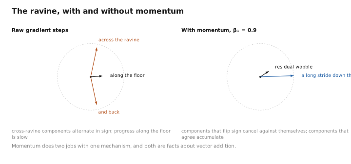
Figure 1. The ravine, with and without momentum.
Per-knob pacing: dividing by how rough the ride has been
The second average addresses scale, and it is the more interesting of the two. Keep a running average not of the gradient but of the gradient squared. Squaring throws away the sign and leaves only size, so what accumulates is not a direction at all but a rough measure of how violently the ground beneath this particular knob has been shifting lately.
Then divide the step by the square root of that quantity. A knob whose gradients have been consistently large has been on rough ground, and its step gets scaled down. A knob that has been quiet for a thousand steps has a tiny running average, so when a gradient finally does arrive, the division makes its step correspondingly long.
This is the trick that makes a single learning rate workable. After the division, the step is no longer measured in raw gradient units — it is measured in units of this knob’s own typical recent gradient. Every knob in the model is put on the same footing, whatever scale it happens to live at, and the learning rate is left to say only how bold we want to be in those normalized units.
A pinch of math: the four lines that make up Adam
Write $g_t$ for the gradient of one knob at step $t$ — the single number backpropagation just handed us. Both running averages are built the same way: mostly the old value, with a splash of the new one.
$$m_t = \beta_1 m_{t-1} + (1 - \beta_1)\, g_t$$$$v_t = \beta_2 v_{t-1} + (1 - \beta_2)\, g_t^2$$The first, $m_t$, is the smoothed direction. With $\beta_1 = 0.9$, each new gradient contributes a tenth and the accumulated past keeps nine tenths, so a consistent pull survives and random jitter cancels. The second, $v_t$, is the same recipe applied to the square, and serves as the roughness meter. With $\beta_2 = 0.999$ it has a far longer memory than $m_t$, which is deliberate: you want your sense of direction to be responsive and your sense of scale to be steady.
Both averages start at zero, which makes them badly wrong for the first few hundred steps, since an average that begins at zero is dragged toward zero. Both are therefore inflated back to honest size by dividing out exactly how much of the average is still made of that initial zero.
$$\hat{m}_t = \frac{m_t}{1 - \beta_1^{\,t}}, \qquad \hat{v}_t = \frac{v_t}{1 - \beta_2^{\,t}}$$At $t = 1$ this multiplies $m$ by ten and $v$ by a thousand; by step ten thousand the correction has faded to nothing. It is bookkeeping rather than a new idea, but without it the opening steps of training are timid in a way that is very hard to diagnose later.
The update itself is then one line:
$$\theta_t = \theta_{t-1} - \eta \cdot \frac{\hat{m}_t}{\sqrt{\hat{v}_t} + \epsilon}$$Read the fraction as direction divided by roughness. The numerator says which way; the denominator says how confidently. The $\epsilon$, usually around $10^{-8}$, is not a dial but a floor — it exists so that a knob with no recent gradient whatsoever does not divide by something vanishingly small and fly off the map. You do not need to hold all four lines in your head at once; the intuition is that Adam is a smoothed direction, rescaled by a smoothed sense of how much this knob has been moving.
Weight decay, and the quiet bug that AdamW fixed
There is one more ingredient, and it comes from a different tradition entirely. Independently of any gradient, it is useful to pull every weight gently back toward zero on every step — a slack elastic tether tied to the origin, doing nothing when a knob is small, tugging harder the further out it drifts. Smaller weights tend to mean smoother functions and better generalization, and they keep the arithmetic tame. This is weight decay, and it long predates Adam.
The traditional way to implement it is to add a penalty on the size of the weights directly to the loss. The optimizer then sees, as part of the gradient, an extra term proportional to the weight itself. With plain gradient descent this is exactly equivalent to shrinking every knob by a fixed fraction each step, which is precisely what we wanted.
With Adam it is not equivalent at all, and the departure is worth savouring. That extra term is now part of $g_t$. It flows into $m_t$, it flows into $v_t$, and — this is the damage — it gets divided by $\sqrt{\hat{v}_t}$ along with everything else. A knob with large, active gradients has a large roughness meter, so its tether is weakened. A knob sitting quietly with tiny gradients has a small roughness meter, so its tether is amplified. The tidying ends up applied in inverse proportion to how busy each knob is, which is close to the opposite of the intent, and it welds the two dials together: change the learning rate and you have silently changed how much decay you are applying.
The fix is disarmingly direct. Do not put the decay in the loss. Apply it as its own separate subtraction, outside the adaptive machinery, after the rescaled gradient step has been computed.
$$\theta_t = \theta_{t-1} - \eta \left( \frac{\hat{m}_t}{\sqrt{\hat{v}_t} + \epsilon} + \lambda\, \theta_{t-1} \right)$$That is the whole of the W — decoupled weight decay, from Loshchilov and Hutter, and the only difference between Adam and AdamW. Every knob is now pulled toward zero by the same fraction regardless of its gradient history, the two dials come apart and can be tuned independently, and models trained this way generalize measurably better. It is a one-line change that took several years to notice, which is a fair summary of how a great deal of progress in this field actually happens.
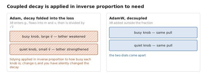
Figure 3. Coupled decay is applied in inverse proportion to need.
What it costs: three copies of the model
Adam’s two running averages are not shared. There is an $m$ and a $v$ for every single knob, which means the optimizer carries two extra numbers per parameter, held at full precision because they accumulate over hundreds of thousands of steps and cannot tolerate rounding.
The full accounting for a large model trained in mixed precision is sobering. Per parameter: two bytes for the half-precision weight used in the forward pass, two for its gradient, four for the full-precision master copy of the weight, four for $m$, and four for $v$. Sixteen bytes per parameter, of which the weights the model actually consists of are two. A seven-billion-parameter model needs about fourteen gigabytes to hold, and about a hundred and twelve to train.
This single fact is why so much of the fine-tuning literature exists. Freeze the base model and you eliminate the master copy, the gradients, and both moments for the overwhelming majority of the knobs — which is precisely the bargain LoRA strikes, and why the frozen base in QLoRA can be squeezed to four bits without touching the small adapter that is still being optimized at full precision. When full training genuinely is required, the usual recourses are to shard the optimizer state across machines so no single device holds all of it, or to keep the moments themselves in eight bits, which turns out to be tolerable in a way that eight-bit gradients are not.
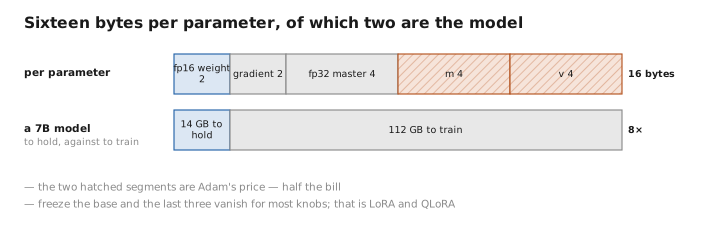
Figure 2. Sixteen bytes per parameter, of which two are the model.
The dials, and what people actually set them to
The learning rate remains the one that matters, and it is almost never held constant. Training opens with a warm-up of a few thousand steps ramping from nearly zero, because Adam’s roughness meter has not yet seen enough gradients to be trustworthy and a confident step taken on a bad estimate can wreck an initialization . It then decays along a cosine curve to something like a tenth of its peak, so that the model finishes with small careful steps.
Of the two betas, the first is essentially always nine tenths. The second is often lowered from the classic $0.999$ to $0.95$ for large language models, which shortens the memory of the roughness meter — with a very long memory the optimizer reacts too slowly to a sudden loss spike, and a model that hits one may take thousands of steps to recover. The decay $\lambda$ is typically a tenth, and is applied to the weight matrices but deliberately not to biases or to normalization gains, which have too few parameters to be worth regularizing and whose natural resting values are not zero anyway. Finally, gradients are usually clipped to a fixed maximum length before the optimizer ever sees them, a seatbelt against the one anomalous batch that would otherwise poison both running averages at once.
What to carry forward
AdamW is what the phrase “the downhill walk” actually means in practice. It keeps two running averages per knob: a smoothed direction, which averages away the noise of mini-batch sampling and lets consistent signals accumulate, and a smoothed roughness, the average squared gradient, which it divides by so that every knob takes a step measured in units of its own recent behaviour rather than in raw gradient units. That division is what allows one learning rate to govern a model whose parameters live at wildly different scales, and it is why Adam works on rare-token embeddings and normalization gains alike. Both averages are bias-corrected in the opening steps, a piece of bookkeeping that matters more than it looks. Bolted on top is decoupled weight decay — a uniform pull of every weight toward zero, applied outside the adaptive rescaling rather than folded into the loss, which keeps the decay from being weakened exactly on the knobs that most need restraining and lets the learning rate and the decay be tuned as independent dials. The price is memory: two full-precision numbers per parameter, which in a full mixed-precision setup means roughly sixteen bytes per knob and an optimizer state several times larger than the model itself. That price is the reason the frozen-base methods exist, and the reason a technique as simple as keeping the moments in eight bits was worth a paper.
The figures in this article follow the shared figure key , which explains what every shape, line style and colour means.
