The cost of running a model is almost always quoted in operations. Training budgets are priced in floating-point operations, architectures are compared by operations per token, and halving the operation count of a component sounds unambiguously like progress. A great deal of work built on that premise produced no speedup, and some of it produced a slowdown. The arithmetic units on a current accelerator stopped being the scarce resource some time ago; they spend most of their existence waiting for numbers to arrive from memory, far more slowly than they can be consumed. Once that gap is wide enough the cost of a computation is set by how much data it touches rather than how much work it does with it, and a cost model counting only the work will misidentify what is expensive with near-perfect reliability. This piece is about the ratio that decides which of the two limits binds, why the same model sits on opposite sides of it in training and in generation, and what that fact explains about everything built on top.
Computing got cheap and fetching did not
The number worth holding onto is a ratio rather than a speed. On a current datacentre accelerator, the arithmetic units can perform something on the order of a few hundred operations in the time it takes to bring one number in from the large memory pool attached to the chip. Not a few. A few hundred.
The gap is no quirk of one design, and it has been widening for decades. Arithmetic is a matter of transistors, which have been getting smaller and more numerous on the familiar schedule; bandwidth is a matter of how many wires run off the edge of a die and how fast each can be driven, a packaging problem that has improved far more slowly. Every generation has added arithmetic faster than it added the means to feed it.
So a chip’s headline figure, operations per second, is available only to computations that arrive with enough data already in hand. Everything else runs at whatever rate memory can supply, and the headline becomes a claim about what the chip could have done. Nearly every performance surprise further up the stack descends from this ratio.
Intensity decides which limit binds
The quantity that settles which limit applies is arithmetic intensity: operations performed, divided by bytes moved to perform them. It belongs to the algorithm and its implementation, not to the hardware.
The hardware supplies its own version of the ratio — peak arithmetic divided by peak bandwidth, the machine balance, which on current parts sits in the region of a few hundred operations per byte. Set the algorithm’s intensity beside it, and whichever is smaller names the wall you are standing against. Intensity comfortably above the balance keeps the units fed and the operation is compute-bound, running near the rated speed. Intensity below it starves them and the operation is memory-bound, running at a fraction of that speed which is, near enough, the ratio of the two numbers.
Drawn out, this is the roofline: attainable performance against intensity, rising in proportion while bandwidth is the constraint, then flattening into a ceiling once arithmetic takes over, with the bend at the machine balance. Where an operation lands tells you what to do about it — below the bend, cut traffic; above it, cut operations. The prescriptions are opposites.
Operation counts are the most quoted measure of cost and frequently the wrong one. A change that halves the arithmetic and doubles the traffic is a slowdown anywhere left of the bend, and whoever made it will have a table showing an improvement. This is the mechanism behind a long run of refinements that were cheaper on paper and no faster in practice: sparse patterns, factorizations, decompositions trading one dense multiply for several small ones. The multiply had been living above the bend, where its operations were nearly free. The replacements moved data instead.
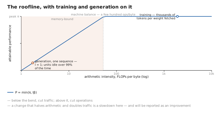
Figure 1. The roofline, with training and generation on it.
Training is compute-bound and generation is memory-bound, and the same model does both
Same weights, same architecture, same chip, two workloads landing on opposite sides of the bend. This is the observation that earns the framework its keep.
A training step pushes a batch of many sequences, each of many positions, through every weight in the model, so a weight matrix is fetched once and then used thousands of times — once per token in the batch — before it is finished with. Intensity is enormous, the units are saturated, and the run is limited by how many operations the chip can perform. Which is why training budgets are quoted in operations, why that quotation is honest, and why scaling laws are written in units of compute.
Generation is the same model in the other regime, and the numbers are startling. To produce one token for one sequence, the model reads every weight out of memory and performs, per weight, one multiply and one add: fourteen gigabytes fetched to carry out roughly fourteen billion multiply-accumulates. An intensity of about one operation per byte, against a machine balance of several hundred — not near the bend but off the bottom of the graph. The units are idle well over ninety-nine percent of the time. They are not computing slowly. They are waiting, and the accelerator is working as an expensive weight-streaming device that multiplies things on the way past.
Two things follow. Single-sequence generation speed is a bandwidth specification: divide the model’s size in bytes by the accelerator’s bandwidth and the time per token falls out, to within a factor that has little to do with the model. And the idle arithmetic is real, paid for, and unspent, on every generation step of every deployment. Most of what follows is people finding ways to spend it.
A pinch of math: operations per byte, and where the batch enters
Write the intensity of a computation as
$$I = \frac{\text{FLOPs}}{\text{bytes}}$$and the machine’s balance, for peak arithmetic rate $\pi$ and peak bandwidth $\beta$, as $B = \pi / \beta$. Attainable performance is the smaller of the two ceilings,
$$P = \min\!\left(\pi,\; I\beta\right)$$which is the roofline in one line: a slope of $\beta$ until $I$ reaches $B$, and a flat $\pi$ thereafter.
Now price the operation that dominates a transformer. Take a batch of $b$ activation vectors of width $d$ against a weight matrix of shape $d \times d$. What has to move is the weight matrix, $d^2$ numbers; the activations are $bd$ numbers, negligible whenever $b$ is much smaller than $d$, which it is. The arithmetic is one multiply and one add per weight per element of the batch, or $2bd^2$ operations. Counting a byte per weight,
$$I = \frac{2bd^2}{d^2} = 2b$$Intensity proportional to batch size, and independent of $d$. The model’s size cancels exactly, which explains the two regimes at a stroke: one sequence gives an intensity of two and is hopeless, a hundred sequences give two hundred and reach the bend, and a larger model changes neither verdict. It also locates the threshold, at half the machine balance — which is why serving systems chase batches of a hundred or two rather than of ten, and why little improves once they are past it.
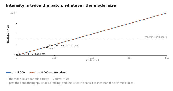
Figure 2. Intensity is twice the batch, whatever the model size.
Most of the serving stack is one observation, restated
Four techniques usually presented as separate inventions, all of them one argument in different clothes.
Batching is the business model. Raising the batch size raises intensity in proportion: the weights are read once and used once per sequence, so the expensive half of the work is amortized while the free half multiplies. Throughput climbs almost without cost until intensity reaches the bend, and then stops. What halts it sooner is not arithmetic but space: the attention cache grows with every concurrent sequence and eats the memory the weights were sharing, which is why scheduling at the granularity of one decode step pays. Serving many users at once is not generosity. It is the only regime in which the hardware is being used at all.
Quantization buys more than its arithmetic saving suggests. Fewer bits per weight means fewer bytes fetched, and bytes are the scarce commodity, so halving a weight’s stored width roughly halves the time per generated token, whether or not the chip supports arithmetic at that width. The saving is in the fetch. Which explains an asymmetry: the same change does much less for training, which sits above the bend where traffic was never the problem, and where mixed precision is chosen for the units it unlocks, not the bandwidth it saves.
Speculative decoding is the idle arithmetic, spent on purpose. Checking five candidate tokens in one pass costs one streaming of the weights, near enough what generating a single token costs, because the extra arithmetic lands in units that were doing nothing. It works only where the surplus exists, which is why it helps a lone user and quietly stops helping a batched server that has spent the same slack on throughput.
Kernel fusion matters because the cheap operations are not cheap. A chain of elementwise steps — scale, add, activate, normalize — has an intensity near one at every link, and an unfused implementation pays a full round trip to memory per link, reading a tensor and writing it back for a few flops per element; fusing the chain into one pass collapses those trips into one. Such operations are a trivial share of a model’s arithmetic and a substantial share of its runtime, and FlashAttention is the ambitious version of the same manoeuvre.
The picture is first-order, and wrong in three known ways. It assumes peak bandwidth is reachable, which requires access patterns the memory system likes; a scattered read achieves a fraction of the quoted figure, so the model quietly overpredicts, and the routing traffic of a sparse model is a standing example. It says nothing about latency, so a small operation can be dominated by launch overhead and reach neither limit. And it treats memory as one thing when there is a hierarchy of pools — exactly the distinction that tiling into fast on-chip memory exploits and the roofline cannot see.
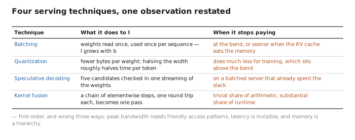
Figure 3. Four serving techniques, one observation restated.
What to carry forward
Arithmetic became cheap faster than bandwidth grew, and on a current accelerator the units can perform a few hundred operations in the time one number arrives from memory. Arithmetic intensity — operations per byte moved — set against that machine balance decides which limit binds: above it a computation is compute-bound, running near its rated speed; below it memory-bound, running at roughly the ratio of the two figures, with the roofline drawing a ceiling that rises with intensity and then flattens. For a batched matrix multiply the intensity is about twice the batch size, independent of model size, which explains the central asymmetry. Training pushes thousands of tokens through each weight it fetches, sits well above the bend, and its cost genuinely is the arithmetic. Generating one token for one sequence reads every weight to perform one multiply-accumulate per weight, an intensity of about one, leaving the units idle over ninety-nine percent of the time. From that number descends most of the inference stack: batching amortizes the weight reads until the attention cache rather than the compute runs out of room, quantization speeds generation by moving fewer bytes rather than doing less work, speculative decoding converts idle units into tokens and stops paying once batching has claimed the same slack, and fusing chains of cheap elementwise operations matters because each unfused link pays a full round trip for a few flops. The framework is first-order and misses three things: peak bandwidth needs access patterns the hardware likes, a small operation can be dominated by launch latency instead, and memory is a hierarchy rather than one pool. What it gets right is which question to ask. A change that halves the arithmetic and doubles the traffic is slower, and it will be reported as an improvement.
The figures in this article follow the shared figure key , which explains what every shape, line style and colour means.
