The gradient the model actually receives is never the gradient of the thing we want to minimize. What we want is the average loss over all text; what we compute is the average loss over a few hundred thousand tokens drawn at random. The second is an estimate of the first, and how many tokens go into it is a choice — the batch size. Larger batches give a cleaner estimate and fewer steps per unit of data; smaller batches give a noisier estimate and more steps. It sounds like a straightforward accuracy-versus-cost trade, and it is not, because the noise turns out to be useful, because the returns from reducing it stop abruptly at a threshold that can be calculated, and because on the hardware these models run on the choice is entangled with how many machines you are using. This piece is about that threshold and what sits on either side of it.
Two things the batch size controls
Separate the two effects at the outset, because conflating them causes most of the confusion.
The first is statistical. Averaging over more samples reduces the variance of the estimate, and it does so in the familiar way: the standard error of a mean over $B$ samples falls as $1/\sqrt{B}$. Quadrupling the batch halves the noise. This is a decelerating return, and the deceleration matters.
The second is mechanical. Every optimizer step costs a fixed overhead — a synchronization across all the machines involved, a gathering of gradients, an update applied to every parameter, a set of communications that do not depend on how much data went into them. Fewer, larger steps amortize that overhead better. On a cluster of thousands of accelerators, the fixed cost of a step is substantial, and there is real pressure to make steps as large as possible so there are fewer of them.
These pull in the same direction up to a point, which is why large-scale training uses batches of millions of tokens. What stops them is that the statistical benefit runs out while the cost does not.
The noise is not simply a defect
Before the threshold, a word about what the noise is doing, because the instinct that a cleaner gradient must be better is wrong.
Gradient descent with a noisy gradient does not walk straight downhill; it jitters. That jitter has consequences that are difficult to characterize precisely but are consistently observed. It shakes the parameters out of narrow crevices in the loss landscape and leaves them in wider basins, and models sitting in wide basins tend to generalize better, plausibly because a wide basin means the loss is insensitive to small perturbations of the weights and therefore, loosely, to small differences between the training data and the world. Very large batches, trained naively, are known to find sharper solutions and to generalize slightly worse than smaller ones at equal data — the “generalization gap” that appeared when people first tried to train with enormous batches to exploit large clusters.
Most of that gap turned out to be fixable by adjusting the learning rate rather than being intrinsic. But the underlying point stands: noise in the gradient is not purely a defect to be minimized. It is a source of implicit regularization, and a training setup that removes it entirely has to replace it with something.
A pinch of math: the critical batch size
The threshold can be derived, and the derivation is the most useful thing here.
Think of the gradient estimate as the true gradient plus noise. The true gradient is what makes progress; the noise contributes nothing on average and merely wastes some of each step. When the batch is small, the noise dominates and averaging more samples buys a great deal. When the batch is large, the estimate is already close to the true gradient and averaging more buys almost nothing — you are paying twice the compute to remove noise that was no longer in the way.
The crossover is where the noise contributes about as much as the signal, and it is captured by a single quantity with units of samples:
$$B_{\text{crit}} = \frac{\text{tr}(\Sigma)}{\|G\|^2}$$where $G$ is the true gradient and $\Sigma$ is the covariance of the per-sample gradients — the numerator measuring how much individual examples disagree with each other, the denominator measuring how strong the consensus direction is. This is the gradient noise scale, and it says something intuitive: the right batch size is set by the ratio of disagreement to agreement among your examples.
Its consequence is a clean statement about diminishing returns. Write $S$ for the number of optimizer steps needed to reach some target loss and $E$ for the total examples processed. Then to a good approximation
$$\frac{S}{S_{\min}} \;=\; 1 + \frac{B_{\text{crit}}}{B}, \qquad\qquad \frac{E}{E_{\min}} \;=\; 1 + \frac{B}{B_{\text{crit}}}$$Read the two together. Below the critical size, doubling the batch nearly halves the number of steps at almost no extra data — steps are cheap to buy. Above it, doubling the batch barely reduces the step count while doubling the data consumed — you are paying in compute for time you no longer save. At exactly $B_{\text{crit}}$ you sit at the corner, using twice the minimum steps and twice the minimum data, which is the balanced point.
So the batch size is not a quality dial at all. It is a dial between wall-clock time and total compute. Below critical, you are wasting time; above it, you are wasting compute. Where you want to sit depends on whether you are short of hardware or short of patience, and organizations training frontier models are generally short of patience and run above critical deliberately.
The noise scale is not a constant. It grows as training proceeds — early on, every example agrees that the model is badly wrong and the consensus is overwhelming, so a small batch suffices; later, the remaining disagreements between examples are what is left to learn from, and a larger batch is needed to hear the signal over them. It grows with model capability for the same reason, and it varies by domain: reinforcement learning has a noise scale orders of magnitude above supervised learning, which is why RL runs use batches that look absurd next to pretraining. This is the honest explanation for a practice that otherwise looks superstitious — ramping the batch size up over the course of a training run, keeping it near critical as critical moves.
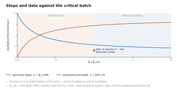
Figure 1. Steps and data against the critical batch.
Coupling to the learning rate
Change the batch size and you must change the learning rate, or you have changed two things at once.
The rule for plain gradient descent is linear: double the batch, double the learning rate, so that the total distance travelled per example stays the same. The rule for a noise-dominated regime is the square root, since that is how the noise falls. In practice, with AdamW , the square-root rule matches observation better across most of the useful range, and the linear rule is the right instinct only when batches are small.
Both rules break at the top. Beyond some learning rate the training becomes unstable regardless of how much data went into each gradient, because the step is simply too large for the curvature of the landscape. This is what caps batch size in practice: past a point, the batch is large enough to support a bigger step but the landscape is not, so the extra data buys nothing at all. The standard mitigations are the warm-up described under AdamW , which lets the optimizer’s running estimates settle before large steps are taken, and gradient clipping, which bounds the damage from an anomalous batch.
Getting a large batch out of small hardware
One practical matter, since the numbers above are unreachable on any single device.
A batch of four million tokens does not fit in the memory of one accelerator, and often not in a thousand. Two mechanisms bridge the gap. Gradient accumulation runs several small forward and backward passes in sequence, adding their gradients into a buffer, and applies one optimizer step at the end — mathematically identical to a single large batch, and trading time for memory. Data parallelism runs the small passes simultaneously on different devices and averages the gradients across them before the step, which is the same arithmetic executed concurrently at the cost of a communication.
Both produce the same update. What differs is the resource spent, and real training runs use both at once: a per-device micro-batch chosen to fill the memory available, multiplied by an accumulation count, multiplied by the number of data-parallel replicas, to reach the target. The consequence worth noting is that the batch size a training run reports is a logical quantity assembled from three separate settings, and that changing the hardware layout without adjusting the others silently changes the optimization.
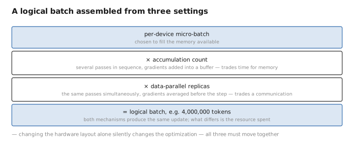
Figure 2. A logical batch assembled from three settings.
What to carry forward
The batch size sets how many examples are averaged into each gradient estimate, and it does two separate things: it reduces the estimate’s noise, which improves as the square root of the batch and therefore decelerates, and it amortizes the fixed overhead of a step, which does not decelerate. Because the statistical return runs out while the mechanical one continues, there is a threshold — the critical batch size, given by the ratio of how much individual examples disagree to how strong their consensus is. Below it, doubling the batch nearly halves the number of steps for almost no extra data; above it, doubling the batch consumes twice the data while barely reducing the steps. So this is not a quality dial but a trade between wall-clock time and total compute, and frontier runs sit deliberately above critical because they are short of time rather than short of hardware. The threshold moves during training, rising as the easy consensus is exhausted and only the disagreements remain, which is the real justification for ramping batch size up over a run, and it is far higher in reinforcement learning than in pretraining. Changing the batch requires changing the learning rate with it — roughly as the square root in the regime that matters — up to a ceiling imposed by the landscape rather than by the data, beyond which no amount of extra averaging permits a larger step. And since no device holds millions of tokens, the reported batch is a logical quantity assembled from a per-device micro-batch, an accumulation count, and a replica count, all three of which must move together to keep the optimization unchanged.
The figures in this article follow the shared figure key , which explains what every shape, line style and colour means.
