Every number in a model is where it is because of one quantity. The loss is what training minimizes, what scaling laws predict, what a training run is monitored by, and what all the machinery of optimization exists to descend. For a language model that quantity is cross-entropy, and it is usually introduced as a formula to be accepted rather than a thing to be understood. That is a shame, because it has an exact and rather beautiful interpretation — it is the number of bits you would waste encoding real text using the model’s beliefs about text — and once that reading is in hand, several otherwise mysterious facts about training curves and model evaluation become obvious. This piece is about what the loss measures, why it and not something simpler, and what its familiar cousin perplexity adds.
The problem with counting mistakes
The obvious way to score a predictor is by accuracy: how often was the top choice correct? For a language model this is close to useless, and for two reasons.
The first is that it is nearly always wrong, and correctly so. Given the cat sat on the, a good model will say mat, but floor, sofa, step, and roof are all perfectly reasonable, and the text may well continue with any of them. A model that assigns mat forty percent and the alternatives sensible shares is behaving well. Accuracy scores it zero whenever the text happened to say floor. Worse, accuracy cannot distinguish that model from one that assigned mat a hundred percent and everything else nothing — a model that is far more confidently wrong, and far worse.
The second reason is fatal for training rather than merely for evaluation. Accuracy is a step function: it does not change at all as a probability moves from 0.1 to 0.4, then jumps the instant the ranking flips. A quantity that is flat almost everywhere has a gradient of zero almost everywhere, and gradient descent has nothing to descend. You cannot train on it.
What is needed is a score that grades the whole distribution, rewards putting mass on what actually happened, punishes confident errors more than tentative ones, and varies smoothly so that any small improvement registers. Cross-entropy is that score, and it turns out to be essentially the only natural one.
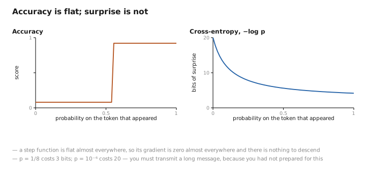
Figure 1. Accuracy is flat; surprise is not.
Surprise, measured in bits
Start from information rather than from statistics. Suppose you believe an event has probability $p$. When it occurs, how surprised should you be?
Whatever the answer, it should have two properties. Something you were certain of should carry no surprise, and something you thought impossible should carry infinite surprise. And the surprise of two independent events together should be the sum of their surprises, since surprise ought to add the way information does — while their probabilities multiply. A function that turns multiplication into addition is a logarithm, and the unique measure satisfying both requirements is:
$$\text{surprise}(p) = -\log p$$Take the logarithm base two and the unit is the bit, with a pleasing concrete meaning: it is the length, in binary digits, of the ideal codeword for an event of probability $p$. Something with probability one-eighth costs three bits to name. Something near-certain costs almost nothing. Something you assigned one chance in a million costs twenty bits — you must transmit a long message, because you had not prepared for this.
The loss of a language model is exactly this, averaged over every token in the data:
$$L = -\frac{1}{N} \sum_{t=1}^{N} \log p_\theta(x_t \mid x_{Why “cross”-entropy
The name comes from a comparison. If text is generated by some true distribution $q$ and you predict with your own distribution $p$, then the average number of bits you spend is:
$$H(q, p) = -\sum_i q_i \log p_i$$This is the cross-entropy of $p$ relative to $q$ — the cost of encoding one distribution’s data using another distribution’s code. The formula above is this quantity estimated from samples, since averaging over observed tokens is averaging over draws from $q$.
The decomposition is where the insight lives. Cross-entropy always separates into two parts:
$$H(q, p) = H(q) + D_{\text{KL}}(q \,\|\, p)$$The first term is the entropy of the true distribution — the irreducible unpredictability of language itself, the cost even a perfect predictor must pay. Text is not deterministic; a great many continuations are genuinely possible, and no model can drive this to zero. The second term is the KL divergence , the extra bits wasted because your beliefs differ from the truth, and it is zero only when they coincide exactly.
Since the first term is a property of language and not of the model, minimizing cross-entropy is precisely and only minimizing the second term. Training is closing the gap between the model’s beliefs and reality, and the loss you observe is that gap plus a constant floor you cannot see and cannot cross.
That floor explains something people find puzzling: loss curves flatten out well above zero and stay there. This is not a failure to converge. A loss of around two nats per token on ordinary English is roughly what an excellent model should report, because language contains about that much genuine uncertainty per token. A model reporting near-zero loss on held-out text has not achieved insight; it has seen the text before.
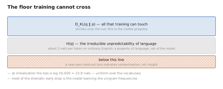
Figure 2. The floor training cannot cross.
What the gradient looks like
There is a practical reason this particular loss pairs so naturally with the softmax , beyond the information-theoretic one, and it is worth seeing because it is unusually tidy.
Composing the two and differentiating with respect to the logits gives:
$$\frac{\partial L}{\partial z_i} = p_i - y_i$$The gradient on each score is simply the probability assigned minus one for the correct token, zero for the rest. Predicted minus actual. Nothing else survives — no factor that shrinks when the model is badly wrong, no term that saturates.
That last point matters more than its simplicity suggests. Squared error composed with a softmax has a gradient containing a factor that vanishes when the output saturates, so a model that is confidently, catastrophically wrong receives almost no correction and can sit there for a very long time. Cross-entropy has no such factor: the worse the error, the larger the correction, without limit. The pairing is not a convention but a genuine mathematical convenience, and it is why implementations fuse the two operations into one function rather than composing them, both for the numerical stability described in the article on logits and because the fused gradient is this single subtraction.
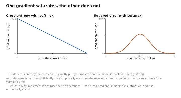
Figure 3. One gradient saturates, the other does not.
Perplexity, and the other units
The same quantity is quoted in several units, and knowing the conversions prevents a lot of confusion.
Reported in nats — natural logarithm — the loss is what appears on a training dashboard, typically falling from around eleven at initialization to somewhere near two. Eleven is not arbitrary: an untrained model spreads probability uniformly over its vocabulary, so its loss is the logarithm of the vocabulary size, and $\log 50{,}000 \approx 10.8$. The first thing any training run does is learn the unigram frequencies, which drops the loss sharply in the opening steps and accounts for most of the dramatic early progress on the curve.
Perplexity is the exponential of the loss:
$$\text{PPL} = e^{L}$$and it has a nice reading. It is the effective number of equally likely options the model is choosing between at each step. Perplexity twenty means the model is about as uncertain as someone picking uniformly from twenty candidates. Because it is exponential, it exaggerates differences at the low end — a fall from 2.10 to 2.00 nats looks small and is a drop from perplexity 8.2 to 7.4 — which is partly why it remains popular, and partly why comparisons using it should be read with care.
The important caveat is that perplexity is not comparable across models with different tokenizers . A model whose vocabulary packs more characters into each token faces fewer, harder predictions and will report a higher perplexity for identical quality. Comparing two models’ perplexities is only meaningful if they cut text the same way. The fix is to normalize by something the tokenizer cannot change — bits per byte, the total surprise over a document divided by its length in bytes — which is why serious cross-model comparisons increasingly report that instead.
What to carry forward
Cross-entropy is the average surprise, in bits or nats, that a model expresses at text that actually occurred: at each position, the negative logarithm of the probability it assigned to the true next token. It replaces accuracy because accuracy grades only the top choice, cannot distinguish a well-calibrated model from a confidently wrong one, and is flat almost everywhere and therefore untrainable. The logarithm is not arbitrary — it is the only function turning multiplied probabilities into added surprise, and it measures the ideal codeword length for an event. The “cross” in the name refers to the cost of encoding one distribution’s data with another’s code, and it decomposes exactly into the entropy of language, which is irreducible, plus the KL divergence between the model’s beliefs and the truth, which is all that training can touch — which is why loss curves flatten out well above zero rather than approaching it, and why a near-zero loss on held-out text indicates contamination rather than excellence. Composed with the softmax it yields a gradient of predicted minus actual, with no saturating factor, so confident errors are corrected in proportion to their size; this is why the two operations are fused in every implementation. And the same number appears as perplexity, its exponential, readable as the effective number of options the model is choosing between — useful, but not comparable across models whose tokenizers cut text differently, for which bits per byte is the honest alternative.
The figures in this article follow the shared figure key , which explains what every shape, line style and colour means.
