A model never produces a word. What comes out of the tower is a set of scores, one per vocabulary entry, and after the softmax a set of odds — a forecast, not a decision. Something outside the model has to read that forecast, commit to a single token, and then do it again, and again, until the text is finished. That something is the decoding strategy, and it is governed by a handful of dials that appear in almost every interface and API you will meet. This piece is about what each of them does, why several of them exist to solve the same problem in different ways, and why not one of them makes a model smarter.
The one thing none of these dials do
It is worth being blunt about this at the outset, because a great deal of confusion follows from getting it wrong. By the time any of these settings takes effect, the model has finished. The forward pass is complete, the distribution over the next token is fixed, and nothing downstream will cause the model to reconsider. Temperature does not make it more imaginative. Truncation does not make it more careful. Every one of these dials is a policy for reading a forecast that has already been issued.
A forecast of seventy percent rain does not tell you whether to carry an umbrella. That depends on how much you mind getting wet against how much you mind carrying an umbrella, and reasonable people with the same forecast make different choices. Decoding parameters are that second decision, and they should be judged the way you would judge any decision rule: not by whether they improve the forecast, which they cannot, but by whether they suit what you are about to do with it.
Two consequences follow, and both matter more than they first appear.
The first is that any deviation from plain sampling is a deliberate distortion. A well-trained model’s distribution is roughly calibrated — it was trained, after all, to match the statistics of real text — so sampling from it exactly is in one precise sense the correct thing to do. We nonetheless almost never do it, because a model that is right about the shape of the distribution can still be wrong in the tail, and because most of the time we want good text rather than representative text. That is a defensible trade, but it is a trade. Nobody is getting something for nothing.
The second is that errors compound. Each token conditions everything after it, so an unfortunate choice does not merely produce one odd word — it leaves the model in a slightly odd state from which the next choice is drawn, and the next. This is made worse by the fact that a model is trained on human text and then asked to continue its own, a discrepancy that widens with every token it generates. Which is why decoding settings barely matter for a three-word extraction and matter enormously for two pages of prose.
Greedy, and why it is worse than it sounds
The simplest possible rule is to take the highest-scoring token every time. It is deterministic, it is reproducible, and it sounds like it ought to be optimal. It is neither optimal nor, for most purposes, good.
The shallow objection is the familiar one about greedy algorithms: the best first step need not lie on the best path. A token that is marginally the most likely here may lead into a region where every continuation is poor, while the runner-up opened onto something far better. Choosing locally and choosing globally are different problems.
The deeper objection is stranger, and it took the field some time to articulate. The most probable sequence is not a typical sequence. Real human text carries a characteristic amount of surprise — writers do not choose the single most predictable word at every opportunity, and text that does so does not read as excellent, it reads as inhuman. Push a distribution over sequences toward its mode and what you find at the peak is very often something nobody would ever write.
In practice this shows up as repetition. Greedy decoding on an open-ended prompt has a marked tendency to fall into a loop, repeating a phrase or a sentence indefinitely, and the reason is a feedback effect the model has honestly learned. Its training data is full of genuine repetition — lists, tables, structured records, code — so it has learned, correctly, that a pattern which has occurred twice is quite likely to occur a third time. Once a phrase has been emitted twice by accident, that machinery fires, the phrase becomes the most probable continuation, and greedy decoding is obliged to take it. Each repetition makes the next more likely. There is no exit.
None of which makes greedy decoding useless. Where there is a canonical right answer — extracting a field, classifying a document, producing code with a conventional form — reproducibility is worth a great deal and the failure mode never arises. It is open-ended generation where it collapses.
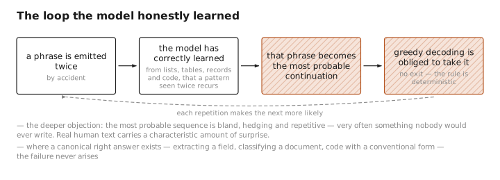
Figure 1. The loop the model honestly learned.
Temperature: flattening and sharpening the field
The remedy is to sample rather than to maximize, and the first dial governs how the sampling is weighted. Temperature divides every logit by a constant before the softmax, which is the same operation described in the article on logits and the same one used, to a completely different end, to soften a teacher’s output in distillation .
Below one, the gaps between scores widen, the leader pulls further ahead, and the distribution sharpens toward the greedy limit. Above one, the gaps close, the field bunches, and at sufficiently high values the model is choosing more or less at random from its vocabulary. Zero is greedy exactly.
It is routinely described as a creativity dial and that description is misleading. Raising the temperature does not supply the model with ideas it did not have; the ranking of candidates is unchanged and no new option is invented. What changes is how far down the existing ranking you are willing to reach. Sometimes the token four places down was the interesting one, and the result reads as inspiration. More often it was ranked fourth for a good reason, and what follows is the model gracefully writing its way around a word it would not have chosen. Both outcomes are the same mechanism.
Two practical notes. Whether temperature is applied before or after truncation differs between implementations, and the two orders give different results — scaling first and then taking the top share of the mass is not the same as taking the top share and then scaling it. It is worth knowing which your stack does. And reasoning models frequently want a specific moderate temperature rather than the lowest available, because they were trained on rollouts sampled at that temperature; running them greedily can measurably degrade them, which surprises people who assume that less randomness is always safer.
Truncation: top-k, top-p, min-p
Temperature reweights the whole vocabulary but excludes nothing, and exclusion turns out to be the more important job.
The reason is arithmetic. A vocabulary has on the order of a hundred thousand entries, and the overwhelming majority of them are absurd in any given context. But absurd is not the same as impossible: assign each a probability of a millionth and the tail collectively holds a non-trivial share of the mass. A small per-token chance of drawing something ridiculous becomes, over a thousand tokens, a near-certainty of drawing it at least once — and by the argument above, one such token does not stay local. Truncation exists to convert “unlikely” into “impossible,” which is a categorically different guarantee.
Three rules are in common use. Top-$k$ keeps a fixed number of the highest-scoring candidates. Top-$p$, also called nucleus sampling, keeps as many candidates as are needed to account for a given share of the probability, so the number kept adapts to the shape of the distribution. Min-$p$ keeps every candidate whose probability is at least some fraction of the leader’s. A fourth, locally typical sampling, is the odd one out: rather than working down from the top, it keeps tokens whose surprise is close to the distribution’s average surprise, on the theory that human text maintains a fairly steady information rate — which means it can discard the most likely token for being too predictable.
A pinch of math: what the three rules actually hold constant
All three do the same two things — keep a subset of the vocabulary, discard the rest, and renormalize what survives so it is once again a set of odds summing to one. They differ only in how the subset is chosen. Order the vocabulary by probability so that $p_1 \geq p_2 \geq \ldots$, and the definitions sit comfortably side by side:
$$S_{\text{top-}k} = \{1, \ldots, k\}$$$$S_{\text{top-}p} = \{1, \ldots, m\} \ \text{ where } m \text{ is the smallest index with } \sum_{i \leq m} p_i \geq p$$$$S_{\text{min-}p} = \{\, i \;:\; p_i \geq \tau \cdot p_1 \,\}$$Read them as three different quantities being held fixed. Top-$k$ fixes the count — exactly $k$ candidates, whatever shape the distribution happens to have. Top-$p$ fixes the mass — however many candidates it takes to reach a given share of the probability. Min-$p$ fixes a ratio to the leader — everything within some factor of the front-runner, and nothing else.
The difference is easiest to see in the case that breaks the first two. Suppose the model is confident: one token at $0.9$, with the remaining tenth of the probability smeared across ten thousand tail entries. Top-$k$ with $k = 40$ admits thirty-nine tail tokens that are collectively nonsense. Top-$p$ with $p = 0.95$ is worse than it looks, because it must keep adding candidates until the running total reaches $0.95$ — and since the leader supplies only $0.9$, it goes on to admit however many thousands of tail tokens are needed to scrape together the missing $0.05$. Min-$p$ with $\tau = 0.1$ admits tokens at $0.09$ or above, which here means the leader alone.
Now flip it. Suppose the model is genuinely torn between two hundred reasonable continuations, each near $0.005$. Top-$k$ discards a hundred and sixty of them for no reason at all. Top-$p$ behaves well. And min-$p$, its threshold now standing at a mere $0.0005$, opens up and lets nearly all of them through.
That is the whole argument for the newest of the three: it tightens automatically when the model is sure and loosens when it is not, because it is the only one that measures anything relative to how peaked the distribution already is. All of them are crude proxies for the quantity genuinely at issue, which is the entropy of the distribution — how much real uncertainty the model is expressing at this position — and none of them measure it directly.
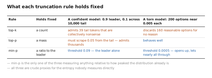
Figure 2. What each truncation rule holds fixed.
Penalties, and why they are blunt
A separate family of dials attacks repetition head-on by penalizing tokens that have already appeared. A repetition penalty scales down the logit of any token seen so far. A frequency penalty subtracts an amount proportional to how many times it has appeared. A presence penalty subtracts a flat amount the moment it appears at all.
They work, in the narrow sense that they reduce repetition. The trouble is that they operate on the identity of individual tokens rather than on the phenomenon anyone actually objects to, which is a degenerate loop. The word “the” will appear a hundred times in any decent paragraph and deserves no penalty whatsoever. A variable name in a program must be repeated exactly, and punishing it produces code that does not run. A list of similar items is repetitive on purpose. These penalties cannot tell any of that apart from a model stuck in a loop, so they tax the good with the bad, and turning them up far enough to stop a determined loop will visibly distort ordinary prose.
There is also a genuine implementation wart worth knowing about. The classic repetition penalty is applied multiplicatively, dividing a seen token’s logit by a factor greater than one. That reduces a positive logit, as intended — but a negative logit divided by a number greater than one moves toward zero, making the token more likely rather than less. The original formulation had to special-case the sign, and implementations that did not do so shipped with the penalty working backwards for exactly the tokens the model was least keen on.
The modern view is that these are patches for a symptom. A capable model with a well-chosen truncation rule loops far less than a weak one, and needs far less penalizing. They remain useful for small models and for particular formats, but reaching for them first is usually a sign that something upstream is wrong.
Beam search, and why chat models abandoned it
Every rule so far commits to one token and moves on. Beam search does not: it keeps several partial sequences alive at once, extends each by every plausible next token, scores the resulting continuations by their total probability, and prunes back to the best handful. It is an attempt to approximate the sequence the model considers most probable overall, rather than the one produced by choosing greedily at each step.
It needs one correction to work. A sequence’s probability is a product of terms below one, so it falls monotonically with length and the search would otherwise always prefer to stop early. Dividing the score by the length, raised to some power, is the standard fix, and that exponent becomes yet another dial.
For a certain class of tasks beam search is genuinely the right tool, and it remains standard in machine translation, speech transcription, and constrained summarization. What those share is that there is approximately one correct output, the model’s probability really does track quality, and the whole exercise is to find the best version of a fixed thing.
For open-ended generation it fails, and the way it fails is instructive. Beam search is not bad at its job. It is good at its job — it reliably finds high-probability sequences — and high-probability open-ended text is precisely the bland, hedging, repetitive material identified earlier as the mode of the distribution rather than a typical draw from it. The better the search, the more thoroughly it locates exactly what you did not want. That is a rare and clarifying kind of failure: the objective was wrong, and improving the optimizer only got you there faster. It is also expensive, multiplying both the computation and the cache by the number of beams.
The dials that are not about choice
Several settings live alongside these without being decision rules at all, and lumping them together causes trouble.
Maximum tokens and stop sequences are control flow. They decide when to halt, not what to say, and the first will cheerfully truncate a sentence in the middle. Stop sequences are matched against text rather than tokens, so a stop string that straddles a token boundary can be missed entirely.
The seed is more interesting than it looks, because fixing it does not actually guarantee identical output from a hosted model. Floating-point addition is not associative, so the order in which partial sums are combined changes the last bits of the result; that order depends on how work is grouped across the batch, and the batch depends on which other requests happened to arrive at the same moment. Two runs with the same seed can therefore diverge, usually harmlessly, occasionally at a position where two candidates were nearly tied. Reproducibility here is best-effort, not a guarantee.
Speculative draft length — how many tokens a small model proposes before the large one checks them — is a pure throughput dial. As described in the article on the KV cache , the verification step provably preserves the large model’s output distribution exactly, so this setting trades wasted draft work against speedup and has no effect whatsoever on quality.
And then there is the thinking budget offered by reasoning models , which belongs in a category of its own. Every other dial here is a different way of reading one distribution. This one causes more distributions to be produced — more tokens of deliberation before the answer begins — and it is the only setting on the list that genuinely buys capability rather than trading one property for another. That it appears in the same settings panel as temperature is an accident of interface design, not a family resemblance.
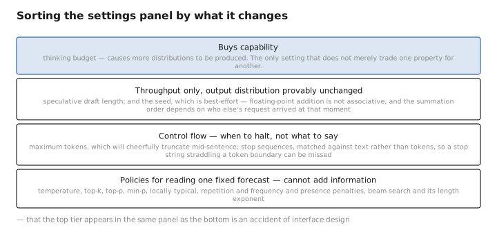
Figure 3. Sorting the settings panel by what it changes.
What to carry forward
A model’s output is a distribution, never a word, and every decoding parameter is a policy for collapsing that forecast into a choice — none of them changes what the model believes, and none can add information that was not in the distribution already. Plain sampling is in a strict sense the faithful thing to do, so every dial that departs from it is trading calibration for something else, and because each token conditions the next, those departures compound over a long generation. Greedy decoding fails on open-ended text not through bad luck but because the most probable sequence is not a typical one, and because the model’s honest belief that repeated patterns repeat again becomes a loop with no exit. Temperature rescales the gaps between scores and controls how far down the ranking you will reach; it invents nothing. Truncation is the more consequential intervention, since it converts unlikely into impossible, and the three common rules differ in what they hold fixed — top-$k$ a count, top-$p$ a share of the mass, min-$p$ a ratio to the leading candidate, with only the last automatically tightening when the model is confident. All are rough stand-ins for the entropy nobody measures directly. Penalties suppress repetition by taxing token identity rather than the pathology, so they punish a variable name and a stuck loop alike, and are best understood as patches for a weak model or a poor truncation setting. Beam search still wins where one right answer exists, and fails at open generation exactly because it succeeds at finding high-probability text. And of the remaining settings, most are control flow or throughput; the thinking budget is the sole exception, and the only dial in the panel that makes the model better rather than merely different.
The figures in this article follow the shared figure key , which explains what every shape, line style and colour means.
