Nearly every language model in use writes the same way: one token, then the next, each conditioned on everything before it and on nothing after. That constraint is so fundamental it is easy to mistake for a fact about language rather than a choice about architecture. It is a choice, and it has costs — a model cannot revise a word it has already committed to, cannot plan the end of a sentence before writing its beginning, and must spend one full forward pass per token no matter how obvious the token is. Image generation abandoned sequential production years ago in favour of starting with noise and refining the whole canvas repeatedly. This piece is about what happens when the same idea is applied to text: why the translation is harder than it looks, what the working version actually does, and why the results are interesting without yet being decisive.
Why the image recipe does not transfer
Diffusion over images works by adding a little Gaussian noise at a time until the picture is static, then training a network to reverse one step of that process. The whole construction rests on the data being continuous: you can add half a unit of noise to a pixel and get a slightly different pixel, and the path from a clean image to pure noise is a smooth one along which every intermediate point is a valid image.
Text is discrete. There is no token halfway between “cat” and “dog”, and adding Gaussian noise to a token index produces something that is not a token at all. The smooth corruption path that diffusion needs does not exist.
The obvious workaround is to run the diffusion in the continuous space of embeddings , where vectors can be noised, and round back to tokens at the end. This was tried extensively and works poorly. The embedding space is mostly empty — real tokens occupy a sparse scatter of points, and a noised vector lands in the vast space between them, where the rounding step is arbitrary and small differences in the vector produce completely different tokens. The geometry that makes diffusion work for images is absent.
Corrupting by masking instead
The construction that works replaces noise with erasure. Rather than degrading a token toward static, degrade it toward absent.
The forward process replaces each token independently with a special mask symbol, with a probability that rises from zero to one over the corruption schedule. At the start the sentence is intact; partway through, some fraction is masked; at the end everything is masked and no information remains. This is a valid corruption path, it is entirely discrete, and every intermediate state is a legitimate partially-observed sequence.
The reverse process is then: given a partially masked sequence, predict what belongs in the masked positions. The model is trained on exactly that — sample a masking rate, apply it, and ask the model to recover the original at every masked position, scored with ordinary cross-entropy .
Anyone who has read about encoder models will recognize this immediately. It is masked language modelling, the objective that trained BERT, with one crucial change: BERT masked a fixed small fraction, around fifteen percent, while this masks a variable fraction drawn across the whole range from nothing to everything. That single difference converts a representation-learning objective into a generative one, because a model that can fill in a sequence which is one hundred percent masked is a model that can write from nothing.
Generation runs the process backwards. Start with everything masked. Run the model, which produces a distribution for every position at once. Unmask some of them — typically those the model is most confident about — and leave the rest masked. Run again, now conditioned on what was just filled in. Repeat until nothing is masked. The whole sequence is produced in a number of steps that is chosen rather than dictated by the length.
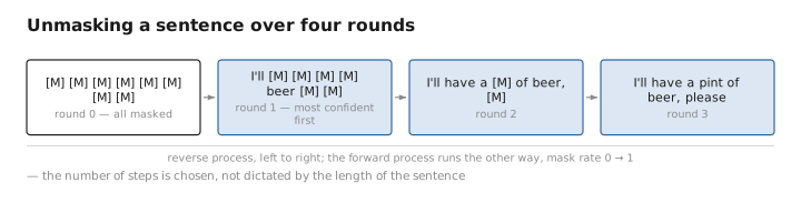
Figure 1. Unmasking a sentence over four rounds.
What this buys
Four properties follow from generating in parallel, and they are genuinely different from what an autoregressive model offers.
Steps are decoupled from length. A sequence of a thousand tokens can be produced in fifty passes rather than a thousand. Whether that is faster depends on the parallelism available, but the scaling is different: doubling the output length need not double the number of model invocations.
Revision is possible. A token filled in early can be masked again in a later round and reconsidered in the light of what has since been written. Autoregressive generation has no mechanism for this at all — a committed token is permanent, and everything after it must be written around any mistake. This is the most structurally significant difference.
Conditioning is bidirectional and arbitrary. Filling a gap in the middle of a document, with fixed text on both sides, is the native operation here rather than an awkward special case. Infilling, editing, and constrained generation with fixed anchors all fall out of the training objective directly.
Planning is not sequential. Because the model sees the whole sequence at every step, it can settle the shape of a sentence before its contents, which is closer to how the constraint-satisfaction aspects of writing actually feel — and it is measurably better on tasks with strong global structure, such as puzzles whose constraints span the whole answer.
A pinch of math: the cost of unmasking in parallel
The central difficulty has a clean statement, and it explains why the step count cannot simply be lowered to one.
At each round the model produces a distribution for every masked position independently, conditioned on what is currently visible. If we unmask $k$ positions at once, we are sampling each from its own marginal:
$$\prod_{i \in S} p(x_i \mid x_{\text{visible}})$$But the correct object is the joint distribution over those $k$ positions:
$$p(x_{i_1}, \ldots, x_{i_k} \mid x_{\text{visible}})$$and these are equal only if the positions are conditionally independent, which adjacent tokens in a sentence emphatically are not. Consider the blanks in “I’ll have a __ __” where the model’s marginals put weight on both “hot dog” and “cold beer”; sampling independently permits “hot beer”, which neither marginal disfavours and the joint would have ruled out.
This is exactly the cost of parallel generation, and it is why the number of steps matters. Unmask one position per round and you have recovered autoregression, with the joint respected exactly and no speed gain. Unmask everything in one round and you get incoherence. In between, every round conditions on what the previous round revealed, which repairs the dependencies incrementally — more rounds, better joint, slower generation. The quality-speed dial in a diffusion language model is precisely a dial on how much conditional dependence you are willing to ignore per step, and the strategy of unmasking the most confident positions first is a heuristic for choosing the ones where the marginal is closest to the joint.
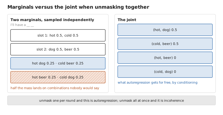
Figure 2. Marginals versus the joint when unmasking together.
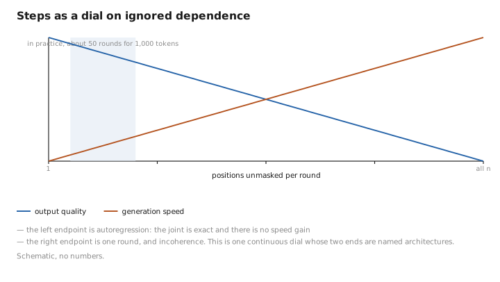
Figure 3. Steps as a dial on ignored dependence.
Where it stands
Models of this kind now exist at meaningful scale — several billion parameters, trained on trillions of tokens — and they are close to autoregressive models of comparable size on standard benchmarks without matching the best of them. That is a substantial achievement given how much less total effort has gone into the approach, and it is not yet a reason to switch.
Two honest problems remain. The first is the KV cache , or rather its absence. Autoregressive generation caches keys and values because the past never changes; in a diffusion model every round can alter any position, so the cache is invalid and the whole sequence must be reprocessed each round. A fifty-step generation is fifty full passes over the entire sequence, which erodes much of the theoretical speed advantage. Approximate caching schemes that reuse work for positions unlikely to change are an active area and are, unavoidably, approximations.
The second is that the entire ecosystem assumes autoregression. Speculative decoding, cache management, the serving stacks, the post-training recipes — all of it is built for one token at a time, and a diffusion model inherits none of it.
The most likely near-term outcome is not replacement but combination: diffusion-style parallel drafting with autoregressive verification, or hybrid models that produce blocks in parallel and sequence the blocks. What the line of work has already established is worth keeping regardless of where it lands — that left-to-right generation is a design decision rather than a necessity, that its inability to revise is a real cost rather than an acceptable one, and that the tokens-equals-forward-passes equation can be broken.
What to carry forward
Diffusion language models abandon left-to-right generation for a process that produces the whole sequence at once and refines it over a chosen number of rounds. The image recipe does not transfer directly, because text is discrete and there is no token halfway between two tokens; running the diffusion in embedding space fails because real tokens are a sparse scatter and a noised vector lands in the empty space between them. The construction that works replaces noise with masking — corrupt a sequence by replacing tokens with a mask symbol at a rate swept across the full range from none to all, and train the model to recover them, which is masked language modelling with a variable rather than fixed rate, and that one change makes the objective generative. Generation starts fully masked and unmasks progressively, usually the most confident positions first. What this buys is real: steps decoupled from output length, the ability to revise a token already written, native infilling with fixed text on both sides, and non-sequential planning that helps on globally constrained tasks. The central cost is precise — unmasking several positions at once samples each from its own marginal while correctness requires the joint, and those differ whenever tokens are dependent, which is why fewer steps means more incoherence and why the step count is exactly a dial on how much conditional dependence is being ignored. Current models are close to autoregressive ones of similar size without surpassing them, they cannot use a KV cache because any position may change in any round, and they inherit none of the ecosystem built around one-token-at-a-time generation — which makes hybrid arrangements the likely near-term outcome, and leaves the durable contribution as the demonstration that sequential generation was a choice all along.
The figures in this article follow the shared figure key , which explains what every shape, line style and colour means.
