There is a boundary running through post-training. Where an answer can be checked by a program, verifiable rewards give a training signal that cannot be flattered, and we can push on it as hard as we like. But most of what we ask a model to do has no checker. There is no program that decides whether an explanation was pitched correctly, whether a refusal was gracious, whether a summary kept the right things. For that territory — which is most of the territory — we are back to human preference, and the standard way of learning from it is a three-stage apparatus with a reinforcement learning loop at the end. Direct preference optimization is the discovery that the whole apparatus collapses into a single loss you can train the way you train anything else. This piece is about how something that looks like reinforcement learning turns out, on inspection, to be classification.
The three-stage machine, and what each stage costs
The conventional pipeline runs like this. First, fine-tune the base model on curated demonstrations, giving something that answers questions rather than continuing them. Second, collect pairs of responses to the same prompt, ask people which they prefer, and train a separate network — the reward model — to predict those judgements. Third, run reinforcement learning: let the model generate, score each generation with the reward model, and update toward higher scores, with a penalty on how far the model’s output distribution is allowed to drift from where it started.
It works, and it produced every assistant you have used. But look at what the third stage requires resident in memory at once. The model being trained. A frozen copy of where it started, needed to compute the drift penalty. The reward model, doing the scoring. And, if you are using the standard algorithm , a critic network estimating how good a partial generation is likely to turn out. Four models, of which two or three are the size of the one you actually want. Inside the training loop there is a sampling loop, because the model must generate its own material to be scored on, and generation is slow. The whole arrangement has a reputation for instability and carries a long tail of hyperparameters that interact with each other in ways nobody finds intuitive.
And hanging over it is the problem that dogs every reward model: it is a proxy, it can be satisfied without the underlying preference being satisfied, and the drift penalty exists precisely to stop the model from finding the places where the proxy is most wrong. The leash is not a refinement. It is load-bearing.
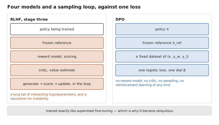
Figure 1. Four models and a sampling loop, against one loss.
What is the reward model actually for?
Step back and notice the shape of the pipeline, because the question almost asks itself.
We start with data: a pile of triples, each one a prompt, a response people preferred, and a response they did not. We finish with a policy: a model that behaves the way those people wanted. In between we build a reward model, which is a compression of the preference data into a network, and then we spend an expensive reinforcement learning phase querying that network to recover what we compressed into it.
The reward model, in other words, is an intermediate. Nothing about the final product requires that it exist — it exists because reinforcement learning wants a reward function, and preferences are not a reward function. It is a translation step, performed so that the next stage can consume its output, and like any translation it loses something on the way through.
So the question is whether the translation can be skipped: whether there is a path from preference pairs directly to a policy, with nothing in between. There is, and the route to it runs through a piece of algebra that has been sitting in plain sight since the objective was first written down.
A pinch of math: the reward hiding inside the policy
The thing reinforcement learning from human feedback is trying to maximize is this: high reward on average, minus a penalty proportional to how far the policy $\pi$ has strayed from the reference $\pi_{\text{ref}}$ it started at, with $\beta$ setting how tight the leash is.
It is a standard result — and the derivation is short, though we will not do it here — that this objective has an exact optimum, and that the optimum can be written down in closed form:
$$\pi^*(y \mid x) = \frac{1}{Z(x)}\, \pi_{\text{ref}}(y \mid x)\, e^{\,r(x,y)/\beta}$$Read it as a statement about reweighting. The best possible policy is the model you started with, with every response’s probability multiplied by the exponential of its reward, then renormalized so the whole thing still sums to one. High-reward responses are made more likely in proportion to how good they are; the reference distribution supplies everything else. The $Z(x)$ is that renormalization, and it is hopeless to compute, since it requires summing over every response that could ever be written.
Here is the move. That equation relates a reward to a policy — so turn it around and solve for the reward instead:
$$r(x,y) = \beta \log \frac{\pi^*(y \mid x)}{\pi_{\text{ref}}(y \mid x)} + \beta \log Z(x)$$Which says something quite striking. Any policy is implicitly the optimal policy for some reward function, and that reward function can be read directly off the policy: it is how much more likely this policy makes a response than the reference did. No separate network is needed to hold a reward, because a model that has a reference to be compared against already is one.
That is the insight, and there remains one obstacle: the intractable $Z(x)$ is still sitting there. It disappears for a reason worth savouring. The standard model of how a human converts two options into a preference — the Bradley–Terry model, borrowed from the statistics of paired comparisons — says the probability of preferring $y_w$ over $y_l$ depends on the difference of their rewards, passed through a logistic curve. Both responses answer the same prompt $x$, so both carry the same $\beta \log Z(x)$ term, and in a difference it cancels exactly.
What is left, after substituting the expression above into Bradley–Terry and taking the negative logarithm, is the entire method:
$$\mathcal{L} = -\log \sigma\!\left( \beta \log \frac{\pi_\theta(y_w \mid x)}{\pi_{\text{ref}}(y_w \mid x)} \;-\; \beta \log \frac{\pi_\theta(y_l \mid x)}{\pi_{\text{ref}}(y_l \mid x)} \right)$$You do not need to have followed every step; the thing to carry away is what the final line contains and what it does not. It contains the model being trained, a frozen reference, a preferred response, a rejected one, and a single dial. There is no reward model anywhere in it, no sampling, no critic, no reinforcement learning of any kind. It is a logistic loss over pairs — the same object you would write down for an ordinary binary classifier — and it is trained by feeding it a fixed dataset, exactly like supervised fine-tuning.
There is a pleasing echo here of something from the article on logits . A single log-probability, quoted alone, is not a reward and cannot be one; there is no fixed zero on that scale. But a ratio against a reference is perfectly well defined, in the way that an altitude is meaningful once someone agrees on sea level. DPO’s reward is a measurement taken against a benchmark, and the benchmark is the model you began with.
What the loss is actually doing
The gradient is worth a paragraph, because it makes the behaviour concrete.
Differentiating that loss gives an update that raises the log-probability of the preferred response and lowers the log-probability of the rejected one — no surprise — multiplied by a coefficient that is large exactly when the model’s implicit reward currently has the pair ordered backwards. A pair the model already scores correctly, by a comfortable margin, produces a coefficient near zero and contributes almost nothing to the update. A pair it gets confidently wrong dominates.
So the training automatically concentrates on its own mistakes, which is a property the reinforcement learning version has to work harder for. And the reference model earns its place twice over: it defines the scale on which the implicit reward is measured, and by appearing in both log-ratios it keeps the policy anchored. The leash is not bolted on as a separate penalty term here. It is structural — a consequence of the reward being defined as a ratio to the starting point in the first place.
The dial $\beta$ has the same meaning it had in the original objective. Small values loosen the leash and let the model move a long way to satisfy the preferences; large values keep it close to where it started. It is the one hyperparameter that genuinely matters, which after the tuning burden of the three-stage pipeline feels like a gift.
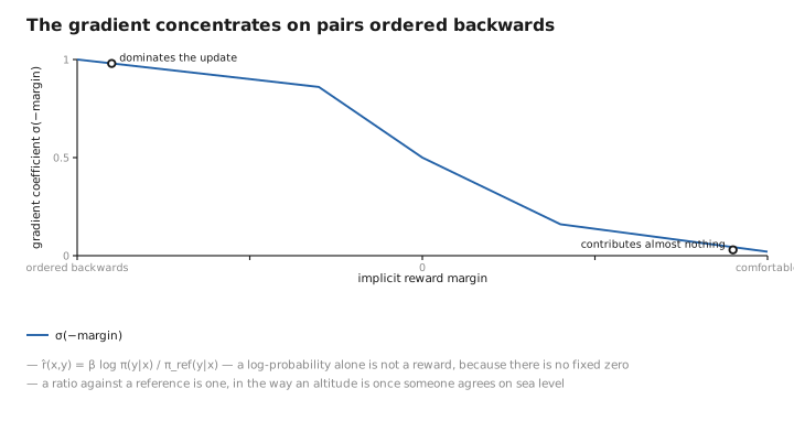
Figure 2. The gradient concentrates on pairs ordered backwards.
Two things the shortcut costs you
It would be dishonest to present this as free, and the two costs are both real.
The first is that DPO is off-policy. The preferred and rejected responses in the dataset were written by someone or generated by some other model, at some point in the past. Reinforcement learning, whatever its expense, has the model generate its own candidates and learn from feedback on those — it is always learning about the region of response space it actually occupies. DPO instead learns from a fixed pile of examples that may be nothing like what the current model would produce, and it is being asked to lower the probability of rejected responses it would never have generated anyway. As training proceeds and the policy moves, the gap between the dataset’s distribution and the model’s own widens, and the signal becomes correspondingly less relevant. This is the main theoretical objection, and it is why the supervised fine-tuning phase beforehand matters more than it looks: the closer the reference model is to the distribution the preference data was drawn from, the less severe the mismatch.
The second is stranger, and was noticed only after the method was in wide use. In practice the log-probability of the preferred response usually goes down during DPO training. Not just the rejected one — both. What rises is only the margin between them, which is all the loss ever asked for. The loss is perfectly satisfied by making the rejected response much less likely and the preferred response merely somewhat less likely, and gradient descent, being indifferent to our intentions, frequently takes that route. The probability mass has to go somewhere, and it flows to responses that appear nowhere in the training pair — sometimes harmless, sometimes not. This is likelihood displacement, and it is the mechanism behind a family of odd failures: models that become terser and terser, or that drift toward a bland register that was never anybody’s preferred answer, or that in the worst reported cases shift mass from a preferred refusal onto a compliance nobody wanted. The margin was the wrong thing to have optimized alone, and nothing in the objective says otherwise.
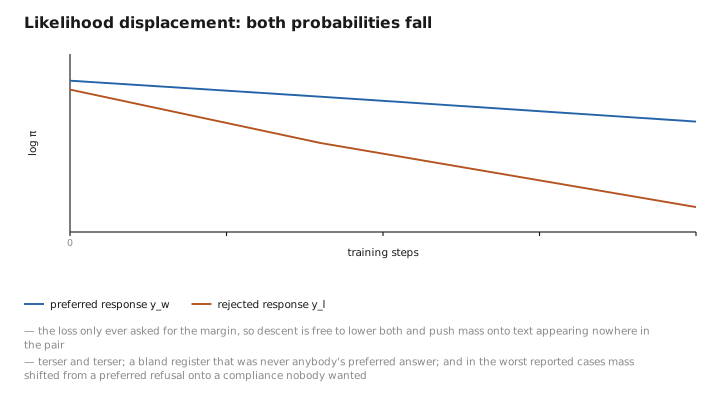
Figure 3. Likelihood displacement: both probabilities fall.
The family that grew around it
Both problems have attracted fixes, and the result is a small ecosystem rather than a single method.
Several variants change the objective’s shape. One line of work observes that when preferences in the data are effectively deterministic — every annotator would agree — the logistic loss can be driven toward an unbounded margin, overfitting badly, and replaces it with a bounded alternative that cannot run away. Another abandons pairs entirely and learns from responses individually labelled good or bad, which is a far easier thing to collect at scale than matched comparisons. Others remove the reference model altogether, either by folding the preference term into the supervised fine-tuning loss so the two happen at once, or by using a length-normalized average log-probability as the implicit reward directly, which has the side benefit of attacking the verbosity bias that afflicts every preference method.
The most conceptually direct fix is to make the method less off-policy: sample fresh responses from the current model, have them ranked — by people, or increasingly by a stronger model acting as judge — and run DPO on those, then repeat. Iterating in this way recovers much of what on-policy training provides while keeping each round cheap and stable. It has become the default recipe for open-weight post-training, and it is a fair description of what most people now mean when they say they are doing DPO.
Where all this sits relative to verifiable rewards is worth stating plainly, because the two methods are complements rather than rivals. Verifiable rewards apply where a checker exists and permit very aggressive optimization; preference methods apply everywhere else and are inherently limited by the fidelity of a proxy. A modern pipeline uses both — preference optimization for helpfulness, tone, formatting, and safety, verifiable rewards for mathematics, code, and reasoning — and the reason DPO in particular became ubiquitous is not that it beats a well-tuned reinforcement learning setup on quality. It is that it removes three models from memory and most of the hyperparameters from the problem, which put a capability that had belonged to a handful of large labs within reach of anyone with a preference dataset and a single machine.
What to carry forward
DPO replaces the reward-model-plus-reinforcement-learning half of preference training with one supervised loss. The step that makes it possible is the observation that the usual objective — maximize reward, stay near a reference — has a closed-form optimum, which can be inverted to show that any policy already is a reward model: its implicit reward for a response is $\beta$ times the log of how much more likely it makes that response than the reference does. Feed that expression into the Bradley–Terry model of preference and the intractable normalizing term cancels, because a preference depends only on the difference between two rewards for the same prompt, leaving a plain logistic loss over chosen and rejected pairs with no reward model, no critic, no sampling loop, and one dial. Its gradient weights each pair by how badly the model currently has it ordered backwards, so training concentrates on its own errors, and the leash to the reference is structural rather than an added penalty. The costs are that it is off-policy, learning from a fixed dataset that drifts further from the model’s own behaviour as training proceeds, and that it optimizes only the margin — so the preferred response’s probability commonly falls too, with the displaced mass landing on text nobody chose. The variants that followed either bound the objective, drop the pairing requirement, remove the reference model, or restore on-policy sampling by regenerating and relabelling each round; that last recipe is now the standard. And the whole family occupies the ground that verifiable rewards cannot reach — everything about a model’s behaviour that no program can check.
The figures in this article follow the shared figure key , which explains what every shape, line style and colour means.
