A model does not see words. Long before the first block of the tower does anything, each token has been replaced by a list of a few thousand numbers pulled from a table with one row per entry in the vocabulary. That table is the embedding, and it is the model’s only point of contact with language as we write it. What is easy to miss is that nobody wrote the table — it begins as noise and is learned by exactly the same downhill walk that trains everything else, with one peculiarity in how the gradient reaches it. What is easier still to miss is that most models keep two such tables rather than one. This piece is about how a word finds its place, and about why reading a word and reaching for a word turn out to be different skills.
The table that begins as noise
The embedding table has one row per vocabulary entry and one column per dimension of the model’s internal arrow. With a vocabulary of a hundred and twenty thousand tokens and a width of four thousand, that is close to half a billion numbers, all of which start out as small random draws.
It is worth dwelling on how empty that starting point is. In a space of four thousand dimensions, random vectors are very nearly perpendicular to one another — not as a curiosity but as an overwhelming statistical fact, since there is so much room that two arrows drawn at random have almost no reason to share a direction. So at initialization the model’s position is not that it has bad ideas about which words are related. It is that it has no ideas at all: every token is as unrelated to every other as it is possible to be. There is no seeded knowledge that " cat" and " dog" belong together, no grammatical categories, no sense that " running" is a form of " run". A linguist could supply all of that in an afternoon, and nobody does.
Everything the table eventually contains is a residue of a single pressure. The tower downstream has to predict the next token, and it is easier for the tower if words that need similar treatment arrive looking similar. Nothing ever instructs the table to group synonyms. Grouping emerges because a row that behaves like its neighbours lets the machinery above it be reused, and reuse is what a limited number of knobs rewards.
A lookup is a multiplication in disguise
Selecting row $t$ from a table looks like an operation of a different kind from anything else in the network — an indexing step, a database query, something outside the arithmetic. It is not, and seeing why explains almost everything that follows.
Write the token as a one-hot vector: a list as long as the vocabulary, zero everywhere except a single one at position $t$. Multiply that vector by the embedding matrix and what comes out is precisely row $t$, because every other row has been multiplied by zero. The lookup is a matrix multiplication whose left operand happens to be mostly zeros.
No implementation actually performs that multiplication — gathering the row directly is a hundred thousand times cheaper, and every framework does exactly that. But the equivalence is the conceptual point. It means the embedding table is not a special structure requiring special handling; it is an ordinary weight matrix sitting at the bottom of the network, and backpropagation reaches it by the ordinary route with no exception carved out for it. It also means the peculiar shape of its gradient is not a design decision anyone made. It is a consequence of all those zeros.
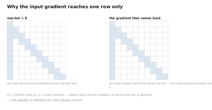
Figure 1. Why the input gradient reaches one row only.
The gradient that only touches what it saw
When backpropagation runs, a message travels down through every block of the tower and arrives at the very bottom, at each position, in the form of a vector saying: the input here should have been a little more like this and a little less like that. That message is the gradient with respect to the embedded vector at that position.
Now push it one step further back, through the one-hot multiplication, to the table itself. Because the one-hot is zero everywhere but one place, the gradient with respect to the table is zero everywhere but one row. The message updates the row for the token that was actually there, and no other row learns anything from that position.
Aggregate this across a batch and the consequence is stark. Each row’s gradient is the sum of the messages from every position where that token appeared — and exactly zero if it appeared nowhere. The token " the" turns up thousands of times in a single batch, so its row collects thousands of messages and is revised on every step of training, from the first to the last. A token that appears once in ten thousand documents collects nothing for thousands of consecutive steps, then receives a single modest message, then falls silent again. Between the busiest and the quietest rows in the table the ratio of update opportunities can run to a million to one.
This is the cleanest example anywhere in a language model of why one global step size cannot work, and it is precisely the situation that per-knob pacing was built for. A rare row’s roughness meter has decayed to almost nothing during its long silence, so when its gradient finally arrives the step it takes is long — the optimizer treats a rare event as informative, which it is.
There is a subtler consequence of the same silence, and it is one people are frequently surprised by. Decoupled weight decay is applied on every step to every parameter, whether or not a gradient arrived. So a rare token’s row is being pulled toward zero on all those thousands of steps when the token is absent, with nothing pushing back. A frequent token’s row is shrunk just as often but is constantly re-inflated by its gradients. Some of the well-known relationship between a token’s frequency and the size of its embedding is not semantics at all; it is a bookkeeping artifact of decaying rows that nobody was updating. Implementations that apply decay only to the rows a batch actually touched behave differently, which is one reason embedding tables are often given their own optimizer settings.
Two maps: reading a word and reaching for one
Everything so far concerns the table at the bottom. There is another at the top.
Recall from the discussion of logits that the final arrow out of the tower is turned into scores by dotting it against a direction belonging to each vocabulary entry. Those directions form a matrix of exactly the same shape as the embedding table — one row per token, one column per dimension. It is usually called the unembedding, and by default it is a completely separate set of numbers, learned independently.
So the model keeps two maps of the same vocabulary, and they answer different questions. The input map answers: when I read this token, what should I contribute to the running state? The output map answers: what must the running state look like for me to say this token? Those are not the same question, and the asymmetry is the same one that separates recognition from production in a person. You can read a great many words you would never reach for; you can recognize a face you could not draw. Reading and producing draw on different information about the same word.
Make it concrete with a word like " the". As an input, what matters about it is almost entirely structural — a determiner has arrived, a noun is probably coming, and the word itself carries close to no meaning. As an output, what matters is something else entirely: what does a state look like just before a determiner is due? The input map needs to encode what the word contributes; the output map needs to encode what predicts it. There is no reason for those to be the same list of numbers, and for function words they are conspicuously not.
The two maps also live in completely different gradient regimes, which is the practical half of the distinction. The input map, as we have seen, is updated sparsely — only the rows that showed up. The output map is updated densely: because the softmax normalizes over the whole vocabulary, every single row participates in every single prediction, and therefore every row receives a gradient at every position. A hundred thousand small corrections per token, against a handful of large ones at the bottom. For a rare word, the input row may go untouched for a week of training while its output row is being nudged several trillion times.
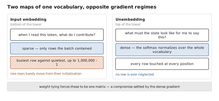
Figure 2. Two maps of one vocabulary, opposite gradient regimes.
A pinch of math: the two gradients
The input side is the simpler of the two. Write $e_t$ for the row belonging to token $t$. Backpropagation delivers, at each position, a vector saying how the input there should have differed. The gradient for $e_t$ is the sum of those vectors across every position in the batch where token $t$ appeared, and nothing at all if it appeared nowhere. That is the whole story, and its shape is the point: a sum over occurrences, and a hard zero otherwise.
The output side is more interesting. The logit for entry $i$ is $z_i = h \cdot w_i$, where $h$ is the arrow the tower produced and $w_i$ is that entry’s row in the output map, and the loss is the negative logarithm of the probability assigned to the token that actually came next. Working the softmax and the logarithm through together — a derivation that simplifies far more than it has any right to — leaves something remarkably clean:
$$\frac{\partial L}{\partial w_i} = (p_i - y_i)\, h$$Here $p_i$ is the probability the model assigned to entry $i$, and $y_i$ is one for the correct token and zero for everything else. You do not need to trace the algebra; the instruction it encodes is the entire training signal for the output map in a single line, and it is worth reading slowly. For the correct token, $p_c - 1$ is negative, so the step moves $w_c$ toward $h$ — the next time this state arises, cast a longer shadow. For every other entry, $p_i$ is positive, so $w_i$ is pushed away from $h$, in exact proportion to how much probability it was wrongly given. The word that nearly won is shoved hard. A word the model already considered impossible is barely moved at all.
Two things follow. The first is the density noted above: every row is touched at every position, and the strength of the touch is that row’s own probability, which is why the output map is shaped mostly by near-misses. The second is that the same quantity, gathered back across the whole vocabulary, is what flows down into the tower:
$$\frac{\partial L}{\partial h} = \sum_i (p_i - y_i)\, w_i$$Read as an instruction to the layer below: point more like the word you should have said, and less like each word you were tempted by, weighted by how tempted you were. Every gradient that trains the entire tower begins as this one vector.
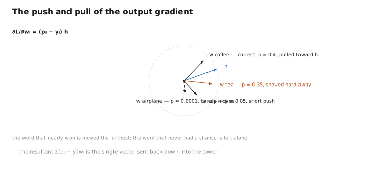
Figure 3. The push and pull of the output gradient.
Tying the two together
Given two matrices of identical shape holding related information, an obvious economy suggests itself: use one matrix for both. This is weight tying, and for years it was close to universal.
The argument for it was partly principled and partly financial. Principled, in that a word’s input and output representations ought to have something to do with each other, and forcing them to coincide is a form of regularization that stops the two from drifting into unrelated encodings of the same thing. Financial, in that when models were smaller the embedding was an enormous share of the total: at half a billion parameters, two untied maps could easily be most of a one-billion-parameter model, and halving that was not a marginal saving. Tying also means a rare token’s row inherits the dense output gradient, so it is being shaped continuously even during the long stretches when the token itself never appears — which, for the tail of the vocabulary, is most of training.
The argument against it is the one made above: the two jobs are different, and a single set of numbers cannot be optimal for both. A tied row is a compromise, and it is not an even-handed one. The output gradient arrives at every step and the input gradient arrives occasionally, so the compromise is settled overwhelmingly in favour of production. The row ends up being mostly an answer to “what precedes this word,” with the reading role fitted around it.
Which consideration wins has shifted with scale. When the vocabulary is large relative to the model, tying is close to free and the regularization is welcome. As models grew, the embedding became a small fraction of the whole, the saving stopped mattering, and the constraint started to cost measurable quality — so the largest models today generally keep the two maps separate, while smaller ones and those with unusually large vocabularies often still tie them. It is a genuine trade rather than a solved question, which is why you will find both in current systems.
What the map actually looks like
It is worth being straight about how much of the popular picture survives contact with a real table, because the folk version is not quite wrong but is oversold.
The famous demonstration — that the arrow from " man" to " woman" is roughly the arrow from " king" to " queen", so that arithmetic on vectors performs analogy — comes from an earlier generation of static embeddings, models like word2vec and GloVe whose entire job was to produce one good vector per word. There, the vector had to be the final word on meaning, and the training objective pushed hard to make the geometry regular. In a transformer’s input table the effect is present but weaker and considerably less reliable, and the reason is structural: the input embedding is not the final word on anything. It is a starting guess that thirty or eighty blocks of attention will refine using context, and a great deal of what we mean by a word’s meaning is assembled up there rather than looked up down here. The input row for " bank" does not have to resolve which sense is intended. It only has to give the tower enough to work with.
Two other features of real tables are worth knowing. Learned embeddings do not spread out to fill the space available to them; they occupy a surprisingly narrow cone, so that two arbitrary tokens have a much higher cosine similarity than intuition suggests. Anyone comparing embeddings directly has to centre or whiten them first, or the similarity scores will be dominated by the shared direction that every token has in common. And frequency leaves a heavy imprint on the geometry — often the single largest axis of variation across the table tracks how common a token is rather than anything you would call semantic, which is a useful thing to remember before reading meaning into a scatter plot.
Finally, the map settles early. Most of the structure in the embedding table is in place within the first small fraction of training, after which the tower above continues to improve for a long time while the table beneath it changes comparatively little. This is a large part of why freezing the embeddings during fine-tuning is usually free, and why so many adaptation methods leave them alone entirely: the map is not where the remaining work is.
What to carry forward
An embedding table is an ordinary weight matrix with one row per vocabulary entry, initialized as noise and learned by the same descent as everything else. Because a lookup is really a multiplication by a one-hot vector, the gradient reaching it is zero for every row the batch did not contain and, for the rows it did, the sum of the messages arriving from each occurrence — so a row’s update frequency tracks its token’s frequency, across a range that can span a million to one. That sparsity is the textbook case for per-knob step sizes, and it also means decoupled weight decay quietly shrinks a rare token’s row throughout its long silences, which accounts for part of the observed link between frequency and embedding size. Most models keep two such maps: an input embedding answering what a token contributes when read, and an unembedding answering what a state must look like for that token to be said. They are different questions, and they are trained under opposite regimes — the input map sparsely, the output map densely, since the softmax makes every row participate in every prediction and pushes each away from the current state in proportion to the probability it was wrongly given. Weight tying merges the two into one matrix, buying parameters and regularization at the cost of forcing one set of numbers to serve both roles, a compromise decided largely by the dense output gradient; it made obvious sense when the embedding dominated the parameter count and is increasingly abandoned as models grow. And the geometry deserves a colder eye than it usually gets: the analogy arithmetic belongs mostly to an earlier era of static embeddings, real tables sit in a narrow cone that inflates every similarity score, frequency rather than meaning is often the largest axis of variation, and the whole map is substantially finished early in training — which is why leaving it frozen during fine-tuning generally costs nothing at all.
The figures in this article follow the shared figure key , which explains what every shape, line style and colour means.
