For a few years the standard illustration of what scale buys you was a plot in which a line lies flat along the bottom of the chart for three or four orders of magnitude and then, past some particular model size, turns upward and climbs almost vertically. The claim attached to it was that the ability being measured is simply absent below that point and present above it — that something switched on. The plot did an enormous amount of work. It appeared in talks about safety, in arguments about regulation, and in forecasts of what the next training run would do. It is also, for a large fraction of the abilities it was drawn for, a property of how the vertical axis was defined rather than of the models along the horizontal one. That does not settle the matter, because a residue survives the objection and the residue is the interesting part. This piece is about what the original claim asserted, the deflationary account that dismantles most of it, and what is left standing.
What was claimed, and why it mattered
The survey that named the phenomenon, from 2022, ran a large collection of benchmark tasks against model scale and picked out a subset with a characteristic shape: performance indistinguishable from chance across every smaller model, then a sharp rise somewhere. Three-digit arithmetic. Multi-step word problems. The term offered for this was emergent abilities, borrowed loosely from the physical sciences, where it names a property of a system that its parts do not have.
Three separate assertions ride inside that one word, and they are almost never argued apart. Unpredictability is the claim that you could not have forecast the ability from smaller models. Discontinuity is the claim that it arrives sharply rather than accumulating. Qualitative novelty is the claim that the larger model is doing something different in kind. These come apart easily. A quantity can be continuous and still unpredictable if all you have measured is its floor, and it can jump on a chart without anything new coming into existence. The bundling is not innocent. The force of the term comes from novelty; the evidence offered is nearly always discontinuity on a plot.
What made the claim land hard was timing. Scaling laws had just established that the pretraining loss of a language model is a smooth power-law function of size, data, and compute, straight on logarithmic axes over many orders of magnitude. Emergence said that the quantity anyone actually cares about, which is what the model can do rather than its cross-entropy on held-out text, does not inherit that smoothness. Loss is forecastable, capability is not. That asymmetry was the entire payload.
The cliff is manufactured by the scoreboard
Here is the objection. It is strong enough that repeating the emergence claim without addressing it is not an argument.
Two different quantities are being conflated. The smooth thing is the model’s loss, a continuous function of the distribution it puts over the next token. The jagged thing is a benchmark score, which is a function applied on top of that distribution — and the function is almost always a threshold. Exact-match accuracy on a multi-step answer pays nothing until every step is right. It is a step function composed with a smooth one, and such a composition can be as sharp as the step is.
Work an example through. Take a task needing five arithmetic steps, scored only on the final answer. A small model gets each step right three times in ten; a larger one, six; a larger one still, nine. The underlying competence has tripled, smoothly, in increments you could have plotted. The exact-match scores are roughly two-tenths of a percent, eight percent, and fifty-nine percent. Flat, flat, cliff. Nothing discontinuous happened inside the model. The discontinuity was made by the scoring rule and then attributed to the thing scored.
The test is to change the ruler and look again. Score the same models on token edit distance to the correct answer, or on the probability they assign to it — a quantity read straight off the logits — or on partial credit per step. Any measure continuous in the outputs rather than thresholded on them. Do this across the tasks originally offered as examples and the cliffs frequently straighten into the curve the loss was already following; for a large share of them the sharpness does not survive the change of metric. That is close to decisive. A property that vanishes when you swap the ruler was a property of the ruler.
And a floor is not a measurement. The rest of the objection concerns resolution. If a score sits at chance for every model below some size, that stretch of the plot records only that the instrument bottomed out. Absence of evidence is being read as evidence of absence. Give the small models credit for partial progress, or sample them enough times to resolve a success rate of one in ten thousand, and they generally turn out to have been improving all along, beneath the resolution of the chart. The flat region was never flat.
The literature was unusually exposed to this. Evaluation of language models runs on thresholded scores — multiple choice marked right or wrong, generation matched against a reference string, code passing or failing a test. A field that measures nearly everything with step functions, then goes looking for steps in its measurements, will find them. The artifact was not a subtle statistical trap. It was the default instrument.
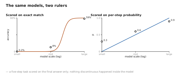
Figure 1. The same models, two rulers.
A pinch of math: what a product of probabilities does to a score
The product argument is worth writing down, because it yields a prediction rather than an alternative story.
Let a task require $k$ steps, each of which the model gets right independently with probability $p$. Exact-match accuracy is the product:
$$A = p^{k}$$Take logarithms and we get
$$\log A = k \log p$$which is linear in $k$. At fixed competence, lengthening a task costs score exponentially. Now let $p$ improve smoothly with scale. For small $k$ the score is as smooth as $p$ is. For large $k$ it stays negligible until $p$ approaches one and then rises steeply, because the sensitivity $dA/dp = k p^{k-1}$ itself vanishes for small $p$ and is largest near $p = 1$. With $k = 10$, moving $p$ from $0.5$ to $0.9$ takes accuracy from about one in a thousand to about one in three. Competence not quite doubled. The score moved by a factor of three hundred.
The prediction follows. The apparent threshold sits wherever $p^{k}$ first clears the benchmark’s noise floor, and that location depends on $k$. So one model family should show its emergence point at different scales for tasks differing only in length, with longer tasks emerging later. That is what is observed — an odd thing if a capability is switching on inside the network, and exactly what to expect if the sharpness lives in the exponent.
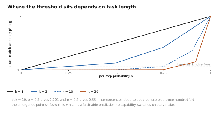
Figure 2. Where the threshold sits depends on task length.
What survives the deflation
The deflationary case is not a proof that behavioural discontinuities cannot happen, and reading it that way is the mirror-image error. It shows that a family of plots does not demonstrate what it was taken to demonstrate. What remains is narrower.
The clean cases are mechanistic rather than metric. The best documented is the formation of induction heads : a two-head circuit that finds where the current token occurred earlier in the context and predicts whatever followed it, assembling over a narrow window of a few hundred optimizer steps. Before that window the model cannot exploit repeated structure. After it, it can. The event shows up outside as a small bump in an otherwise smooth loss curve, and the ability to learn from examples inside a prompt appears at the same moment. The kink is in the cross-entropy itself rather than a thresholded score laid on top, which makes this case immune to the metric objection.
That is emergence over training time, not over scale. The two are routinely conflated, and the conflation flatters the weaker of them. A discrete mechanism assembling at a particular step in a particular run is well evidenced; a capability appearing between one model size and the next is the claim the deflationary argument mostly dissolves. The training-time case is better documented by a wide margin, and it is not evidence for the scale version.
The mechanistic evidence has its own ceiling. The circuit was traced, and switched off by ablation , in small models built for study. At production scale the ablations were never run, so the account there is correlational, and superposition is the reason: components in a large model participate in many circuits at once. Nor is every discontinuity in a loss curve a circuit being born — loss spikes are an optimization pathology with no capability attached, a reminder that a kink is a thing to explain rather than an explanation.
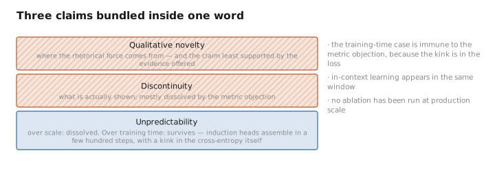
Figure 3. Three claims bundled inside one word.
Both consequences are being acted on at once
The disagreement is not academic: the two readings imply opposite practices and both are in use.
If it is mostly artifact, forecasting is easier than advertised. Then the right move is to pick metrics continuous in the model’s outputs — per-step credit, probability of the correct answer — fit them on small runs, and extrapolate. Capability becomes about as predictable as loss, and the emergence literature was reporting a property of its own scoreboards. Forecasts are now built this way, and it is close to standard practice where planning is required.
If any of it is real, the asymmetry bites. No amount of small-scale testing can rule out a behaviour that shows up only later, because the small-scale measurement may be sitting at the floor. The constraint is one-sided: continuous metrics can raise confidence that a capability will arrive, and cannot establish that one will not. This is the honest reason pre-deployment assessment of a larger model is hard, and why safety cases rest on testing the model actually shipping.
And the axis has stopped being one axis. Reasoning models and test-time compute mean a capability can appear because a system was allowed to spend more work per query rather than because it grew, so “emerges at scale” underspecifies which scale. The word carries three claims and two axes. Splitting it would cost nothing and settle most of the arguing.
What to carry forward
The claim was that certain abilities are absent in smaller models and present in larger ones, arriving abruptly at a threshold rather than accumulating, and what mattered was the consequence: capability would not be forecastable even though loss demonstrably is. The strongest objection is that the smooth quantity is the loss while the jagged quantity is a metric laid on top of it, and metrics like exact-match on a multi-step answer pay nothing until every step lands — so a product of smoothly improving per-step probabilities sits near zero and then climbs steeply while nothing inside the model does anything sharp. Swap to a continuous metric and the cliff frequently straightens; the apparent threshold even shifts with task length, exactly as the product account predicts. A second objection compounds it: a score parked at chance is an instrument at its floor, which is not a measurement, and small models given partial credit usually improve all along. What survives rests on different evidence — a specific circuit assembling over a few hundred training steps, visible as a bump in the loss itself rather than in any scoreboard — and that is emergence over training time, not over scale, which is the conflation to watch for. The dispute is unresolved and both readings are acted on: forecasters choose continuous metrics and extrapolate with reasonable success, while anyone responsible for a frontier model treats small-scale testing as unable to establish absence. The asymmetry is the part to keep. Continuous metrics can tell you a capability is coming; nothing available tells you one is not, and a term bundling unpredictability, discontinuity, and novelty into one word makes that gap easier to argue past than to close.
The figures in this article follow the shared figure key , which explains what every shape, line style and colour means.
