The memory accounting in the article on AdamW left something out. Weights, gradients, and optimizer state came to roughly sixteen bytes per parameter, which is a large number and a fixed one — it does not change with how much text you push through the model. Activations are the other half of the story, and they behave completely differently: they scale with the batch size and the sequence length, and for a large model on a long context they can dwarf everything else. The remedy is one of the more satisfying trades in the whole subject, because it exchanges a resource that is hard and expensive to obtain for one that is merely tedious. This piece is about why the backward pass needs so much stored material, and how throwing most of it away and computing it a second time turns out to be cheaper than keeping it.
Why the backward pass hoards
Backpropagation works by walking the computation graph in reverse, and at every node it needs to know what happened on the way forward.
The reason is the chain rule. To find how the loss changes with respect to a matrix $W$ used in $y = Wx$, you need the gradient arriving at $y$ and the input $x$ that was multiplied by it — the derivative is their outer product. The gradient arrives from above during the backward pass. The input $x$ was computed during the forward pass and, unless it was kept, is gone.
The same is true nearly everywhere. A nonlinearity’s derivative depends on what value passed through it. A softmax ’s backward pass needs the probabilities it produced. A normalization step needs the statistics it computed. So the standard implementation simply stores everything: every intermediate tensor produced during the forward pass is retained until the backward pass has consumed it.
The bill is easy to underestimate. Per layer, per token, a transformer block holds the input to the block, the normalized copy, the query, key and value projections, the attention weights, the attention output, the expanded hidden activation in the feed-forward layer — which alone is four times the model width — and the projection back down. Call it on the order of twenty times the model width per token per layer, in two-byte precision. For a model of width four thousand with eighty layers, processing four thousand tokens, that comes to something in the region of a hundred gigabytes of activations, against a fixed cost of perhaps a hundred and twenty for weights and optimizer state. The activations are not a footnote. They are half the problem, and unlike the fixed half they grow every time you want a longer context or a bigger batch.
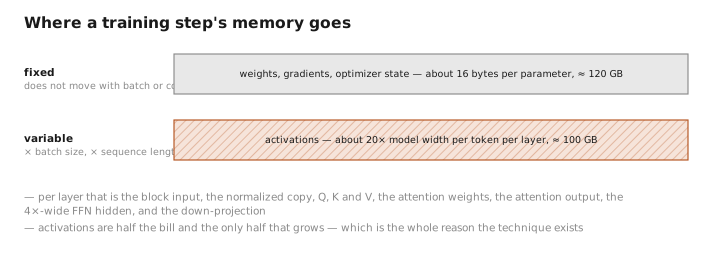
Figure 1. Where a training step’s memory goes.
The trade
Here is the observation the whole technique rests on. The stored activations are not information; they are cached results. Every one of them is a deterministic function of the layer’s input, and could be produced again from that input by running the layer forward a second time.
So do not store them. Keep only a small number of tensors at chosen points in the network — the checkpoints — and discard everything between them. When the backward pass arrives at a discarded region, take the nearest checkpoint below it, run the forward computation again to regenerate the intermediates for that region, use them, and free them immediately.
The cost is one extra forward pass over the recomputed regions. Since a forward pass costs roughly half of a combined forward-and-backward pass, recomputing everything adds about a third to the total compute of a training step — the conventional figure is thirty to forty percent. In exchange, the memory needed for activations falls dramatically.
That is a good trade for a reason worth stating plainly: memory is a hard limit and compute is a soft one. Exceeding memory means the run does not start at all. Exceeding a compute budget means the run takes longer. Anything that converts the first kind of problem into the second is worth a great deal, and thirty percent more time is usually a small price for a model that fits.
A pinch of math: where to put the checkpoints
If you checkpoint every layer, memory is minimal and recomputation is maximal. If you checkpoint none, the reverse. The interesting question is what happens in between, and it has a clean answer.
Take a network of $n$ layers and checkpoint every $k$-th one. Two things then have to be held simultaneously: the checkpoints themselves, of which there are $n/k$, and the activations of the single segment currently being recomputed, of which there are $k$. So the memory required is proportional to
$$M(k) \;=\; \frac{n}{k} + k$$Minimize over $k$ by taking the derivative and setting it to zero, giving $k = \sqrt{n}$ and a memory cost proportional to $2\sqrt{n}$.
This is the result that makes the technique remarkable. Storing everything costs memory proportional to $n$; checkpointing at intervals of $\sqrt{n}$ costs memory proportional to $\sqrt{n}$, while every activation is computed at most twice. An eighty-layer model checkpointed every nine layers holds roughly eighteen layers’ worth of activations rather than eighty, for a single extra forward pass. Depth becomes nearly free in memory terms, which is precisely why models could keep getting deeper.
In practice the granularity is usually coarser and simpler than the optimum suggests — checkpointing at the boundary of every transformer block, which is $k = 1$ in these terms, because block boundaries are the natural place to cut and because the implementation is a one-line change in most frameworks. The theoretical curve matters more when memory is tight enough to require tuning.
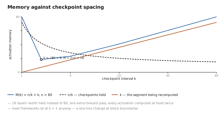
Figure 2. Memory against checkpoint spacing.
Selective recomputation
The uniform version treats every stored tensor as equally worth discarding, and they are not. Two things vary: how much memory a tensor occupies, and how expensive it is to regenerate.
The best candidates are large and cheap. The expanded hidden activation inside a feed-forward layer is four times the model width and is produced by a single matrix multiplication — enormous, trivially recomputed. The output of a normalization step is cheap to redo. Conversely, the attention computation is comparatively expensive to repeat and, with the memory-efficient implementations described under FlashAttention , was never materializing its largest intermediate in the first place.
So modern implementations recompute selectively, discarding tensors ranked by memory saved per unit of recomputation cost, and stopping once they fit. The result is typically most of the memory saving of full checkpointing for a fraction of the overhead — single-digit percentages rather than thirty. Some frameworks do this automatically by profiling the graph; others expose it as a policy to be chosen.
There is also a variant that changes what the extra resource is. Rather than discarding an activation and recomputing it, offload it to the host machine’s ordinary memory and fetch it back when the backward pass needs it. This spends interconnect bandwidth instead of arithmetic, and whether it wins depends entirely on the machine: on a system with a fast link between accelerator and host it can be better than recomputing, and on a system without one it is far worse. The two techniques compose, since a tensor can be offloaded, recomputed, or kept, and the choice can be made per tensor.
Where it sits among the other memory techniques
It is worth placing this against the neighbouring approaches, because they address different parts of the same bill and are routinely confused.
LoRA and QLoRA attack the fixed cost — gradients and optimizer state for parameters that no longer need them, and the storage of the frozen weights themselves. They do very little for activations, since a frozen layer still has to be run forward and, if anything downstream of it is being trained, its output still has to reach the backward pass.
Mixed precision attacks both halves proportionally, by making every number smaller.
Parallelism attacks both by dividing them across machines, and one of its variants is aimed squarely at activations for long sequences.
Checkpointing attacks only the activation half, and it is the only one of the four that spends compute rather than parameters, precision, or hardware. That independence is why it stacks with all of them, and why nearly every large training run has it enabled somewhere in the configuration even when it is not mentioned.
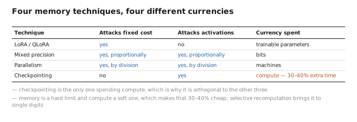
Figure 3. Four memory techniques, four different currencies.
What to carry forward
The backward pass needs, at every node, the values the forward pass produced there — a matrix’s gradient depends on the input it multiplied — so the naive implementation stores every intermediate tensor until it has been consumed. That storage scales with batch size and sequence length, unlike the fixed per-parameter cost of weights and optimizer state, and for a large model on a long context it is comparable to or larger than everything else. But those tensors are cached results rather than information: each is a deterministic function of its layer’s input and can be regenerated. Gradient checkpointing keeps only a sparse set of intermediate points and recomputes the rest on demand during the backward pass, costing roughly one extra forward pass — thirty to forty percent more compute — in exchange for a large reduction in memory. That is a good trade because memory is a hard limit and compute is a soft one: it converts a run that cannot start into a run that is slower. Checkpointing every $\sqrt{n}$ layers of an $n$-layer network is optimal, giving memory proportional to $\sqrt{n}$ with every activation computed at most twice, which is what made great depth affordable; in practice most implementations simply checkpoint at block boundaries. Selective recomputation improves on the uniform version by discarding tensors ranked by memory saved per unit of cost — the fourfold-expanded feed-forward hidden state being the ideal candidate, large and trivially regenerated — recovering most of the saving for single-digit overhead. And the technique is orthogonal to the others, spending compute where LoRA spends trainable parameters, mixed precision spends bits, and parallelism spends machines.
The figures in this article follow the shared figure key , which explains what every shape, line style and colour means.
