Training a neural network is routinely described as finding the settings that minimize a loss, which makes it sound like a search — as though a map existed and the procedure consisted of reading it. There is no map. A model in training has access to exactly one thing: the value of the loss at the point it currently occupies, together with the local slope of that loss in every direction at once. It cannot see the next valley, or tell whether the ground ahead rises or falls. From that poverty of information the entire apparatus of training follows — the tiny steps, the schedules, the momentum, the cautious business of nudging a billion numbers a fraction of a percent at a time. What makes any of it affordable is a piece of arithmetic bookkeeping so efficient it is easy to mistake for a triviality. This piece is about the constraint that only local slope is available, the reverse sweep that recovers that slope for every weight at once, and what the resulting number withholds.
You cannot see the surface you are standing on
Evaluating the loss means running a batch of text through the model and comparing what it predicted against what came next. The result is one number — the cross-entropy , typically between eleven at the start of training and two at the end — covering the current setting of every weight in the tower. It says how wrong the model is here. It says nothing about anywhere else.
The temptation is to picture the loss as terrain seen from above, with training picking a route through it. The view is from the ground, in fog, at night. You feel the slope under your feet and that is the whole of it; there is no vantage point and no survey. Every training run ever performed has been conducted under this restriction.
What the slope buys is a guarantee that holds over an unknown distance: move a small enough step against it and the loss will go down. Small enough is doing a great deal of work in that sentence, and nothing in the slope itself says how small. That omission is the origin of learning rates, warm-ups, schedules , and gradient clipping.
One number that depends on everything
The loss depends on every weight simultaneously, which makes it awkward to picture. A model with a billion parameters defines a function from a billion-dimensional space to one real number, and the object descended is a surface in that space — not a bowl anyone could sketch, a surface whose every point is a complete specification of the model. Geometric intuition trained on three dimensions does not transfer. The algebra does.
For each weight, ask a narrow question: holding every other weight fixed, would a slight increase here make the loss rise or fall, and at what rate. That number is a partial derivative. Collect one per weight and the result is the gradient, a vector with one component per parameter, pointing along the steepest increase. Negate it, step a little way, recompute, repeat. This is gradient descent, and it is not one strategy among several. Given only local slope, it is the only move available.
There is a second poverty layered on the first. The true loss is defined over the whole corpus, and computing its gradient exactly would mean a forward pass over every document to produce one nudge. Nobody does this. It is estimated instead on a mini-batch of a few hundred thousand tokens — unbiased, but noisy: approximately right and locally wrong. That is why batch size is a quality dial and not merely a throughput one, and why a serious optimizer averages the estimate over time.
One sweep instead of a billion
There is an obvious way to compute a partial derivative, and it is worth pricing, because the price is the entire point. Nudge one weight by a tiny amount, run the model forward again, observe how much the loss changed, divide by the nudge. This is a finite difference. It requires no calculus and it works.
It also requires one full forward pass per weight. For a billion-parameter model that is a billion forward passes to obtain the information for a single step, and a training run needs hundreds of thousands of steps. At any plausible speed the arithmetic runs past the age of the universe. Finite differences are not slow. They are hopeless.
Backpropagation obtains all billion partial derivatives in one backward sweep costing roughly twice a forward pass. Not a billion sweeps. One. Deep learning rests on that ratio, and the reason it is available is mundane: the chain rule from first-year calculus, applied in reverse to the graph of operations the forward pass just performed, with intermediate results reused instead of recomputed.
The reuse is where the saving lives. Every weight in layer forty needs to know how the loss responds to layer forty’s output, and that quantity is identical for all of them, so it is computed once. Layer thirty-nine’s version of it is obtained from layer forty’s by one local multiplication. Walk backwards from the loss to the embeddings and each layer is visited exactly once, handing its sensitivity to its predecessor and pairing it with its own inputs to produce its own weight gradients. Nothing is computed twice.
The bill arrives as memory. Producing a layer’s weight gradients requires that layer’s inputs — the activations from the forward pass — so they cannot be discarded as the forward pass moves on. They must be held until the backward sweep collects them, and the quantity held scales as depth times batch size times width, which for a long sequence exceeds the weights themselves. It is the largest consumer of memory in training, and the reason gradient checkpointing exists to trade recomputation against storage.
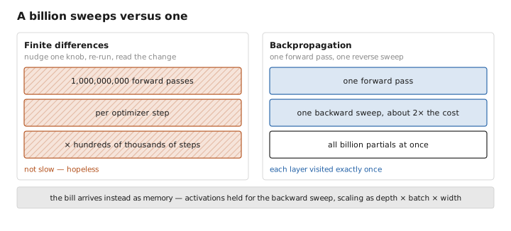
Figure 1. A billion sweeps versus one.
A pinch of math: the chain rule, run backwards
Write the network as a stack of layers, each consuming the previous output along with its own weights:
$$a_n = f_n(a_{n-1}, W_n)$$with $a_0$ the input, $a_N$ the final activations, and $L$ a scalar computed from $a_N$. Now define one quantity per layer, the sensitivity of the loss to that layer’s output:
$$\delta_n = \frac{\partial L}{\partial a_n}$$This is the object the sweep carries; everything else is bookkeeping around it. The chain rule gives two statements, and between them they are the whole of backpropagation:
$$\delta_{n-1} = \delta_n \frac{\partial a_n}{\partial a_{n-1}}, \qquad \frac{\partial L}{\partial W_n} = \delta_n \frac{\partial a_n}{\partial W_n}$$The first propagates. The factor $\partial a_n / \partial a_{n-1}$ is a Jacobian, recording how each output of layer $n$ responds to each of its inputs, and its important property is that it is purely local: it depends on layer $n$’s weights and on what layer $n$ saw, and nothing else. No layer needs to know anything about the layers beneath it to hand back their sensitivity.
The second extracts. Once $\delta_n$ is in hand, the gradient for layer $n$’s own weights is that same sensitivity paired with the layer’s derivative with respect to its weights, which for a matrix multiply is simply the layer’s input. Direction from above, inputs from the side, gradients out.
Now the reason the sweep must run backwards. The recursion builds $\delta_{n-1}$ out of $\delta_n$, so it needs a starting value, and only one sensitivity can be written down directly: the one at the top, where $\partial L / \partial a_N$ follows from the loss and the logits . Nothing comparable exists at the bottom. A symmetric procedure does run forwards, propagating derivatives of one chosen input rather than of one chosen output, at one sweep per input — a billion sweeps for a billion weights, which is finite differences again. Reverse mode costs one sweep per output, and there is only ever one output: many knobs, one number.
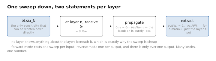
Figure 2. One sweep down, two statements per layer.
What the gradient does not tell you
Four omissions, each with a body of technique attached to it.
It gives a direction and never a distance. The gradient’s magnitude is in units of loss per unit weight, which is not a step size and cannot be converted into one without curvature the gradient does not carry. Multiplying it by a constant is a guess dressed as a hyperparameter. The whole of AdamW — momentum, per-parameter rescaling, decoupled decay — exists to turn a direction into a defensible step length, and the learning rate still sitting on top of it is set by trial.
It contains no curvature. The gradient is a linear approximation to a function that is not linear, valid over a radius it declines to specify. Where the surface bends sharply, a step of the size that worked yesterday overshoots, and the run develops one of the loss spikes that large training jobs are watched for. Second-order methods are well understood; for a billion parameters the object they want is a billion by a billion matrix, which is why they remain an interest rather than a practice.
It requires everything to be differentiable. A gradient reaches back only through operations that respond smoothly to their inputs, so any hard decision inside the model is invisible to training. This has shaped the architecture more than it is credited for: a softmax where a maximum would be the honest operation, soft weighted averages inside attention where selection is what is meant. Where a hard decision is genuinely required, the recourse is to pretend in the backward pass that it was something smoother — a working hack, candid about being one.
It finds a local minimum and claims nothing about the global one. This is the first objection anyone raises, and it matters less than intuition insists. A point of zero gradient is a minimum only if the surface curves upward in all billion directions; if even one curves down, the point is a saddle and descent can leave along it. A billion conditions holding at once is a strong demand, and almost every critical point here is a saddle. Whether that is because most reachable minima are of comparable quality, or because noisy descent from a sensible initialization never comes near a bad one, is unsettled.
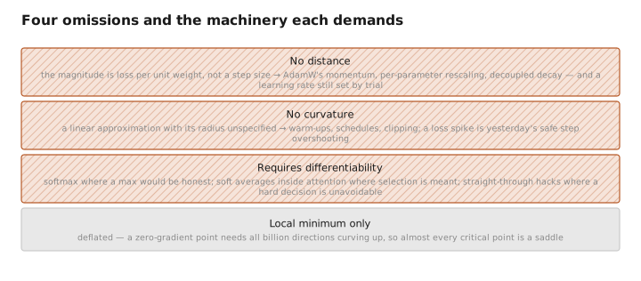
Figure 3. Four omissions and the machinery each demands.
What to carry forward
Training runs under one severe restriction: the loss can be evaluated at the point currently occupied and its local slope measured there, and nothing more. No survey exists, so moving against the slope is not a chosen strategy but the only move on offer. The loss is a scalar function of every weight at once, so the object descended is a surface with as many dimensions as the model has parameters, and the gradient is the vector of partial derivatives pointing along its steepest rise. Recovering it by nudging weights one at a time would cost a forward pass per weight — a billion passes for one step — not expensive but arithmetically hopeless. Backpropagation recovers all of them in one backward sweep costing about twice a forward pass, by applying the chain rule in reverse and reusing each layer’s sensitivity rather than recomputing it; that ratio is why deep learning is possible at all, reverse rather than forward because there is one loss and very many weights. The price is memory, since the backward pass needs the forward pass’s activations, so storage scales with depth times batch times width — the trade gradient checkpointing exists to make. What emerges is narrower than it looks. It is a direction with no distance attached, which is why an optimizer and a schedule are separate machinery; it carries no curvature, so the safe step size is never known in advance; it requires every operation to be differentiable, which has quietly determined what the architecture may contain; and it converges to a local minimum with no guarantee about any other — a weaker complaint than it sounds, since in a billion dimensions almost every critical point is a saddle, though whether the minima actually reached are comparable in quality is still unsettled.
The figures in this article follow the shared figure key , which explains what every shape, line style and colour means.
