QLoRA compressed a frozen model so that adapters could be trained beside it, and mixed precision worked out how few bits a model can be trained in. The third case is the one most people actually encounter: taking a model that is finished and will never be trained again, and making it smaller so that it fits on hardware someone owns. The situation is more forgiving than training, since there are no gradients to preserve and no accumulation to worry about — but it is also less forgiving in one specific way, because there is no opportunity to adapt. Whatever damage the compression does is permanent, and the model must live with it on every request. This piece is about how much can be taken away, why the activations turn out to be harder than the weights, and what the resulting formats actually buy.
Why bother, precisely
The motivation is not storage. It is the bandwidth argument that has now appeared several times: generating a token requires streaming every weight out of memory, and the rate at which that can be done sets the speed. Halve the size of the weights and you halve the traffic, and since the arithmetic units were idle anyway, you approximately double the generation speed. Quantization is a throughput technique that happens to also reduce memory.
The memory reduction is what determines feasibility, though. A model in half precision needs about two bytes per parameter, so a seventy-billion-parameter model wants a hundred and forty gigabytes and does not fit on any single accelerator. At four bits it wants thirty-five, which fits on one. The difference is not incremental; it is the difference between needing a multi-device server and needing a workstation, and it is why quantization is the single technique most responsible for open-weight models being usable by individuals.
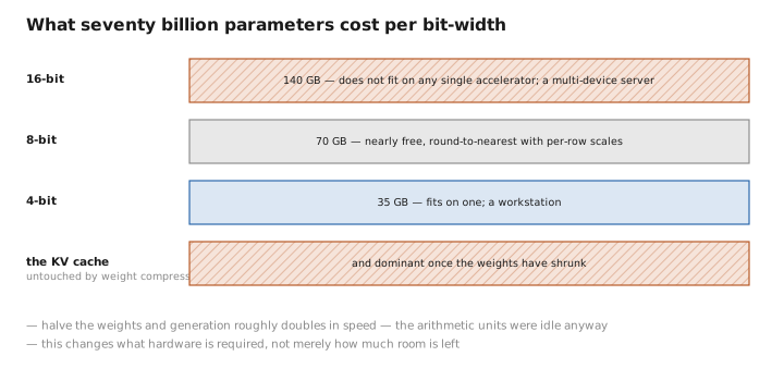
Figure 1. What seventy billion parameters cost per bit-width.
Rounding a weight matrix
The basic operation is the same as in QLoRA. Take a group of numbers, find their range, divide that range into a small number of levels, and record which level each number is nearest to along with the scale needed to recover it.
$$w \;\approx\; s \cdot \text{round}\!\left(\frac{w}{s}\right), \qquad s = \frac{\max|w|}{2^{b-1} - 1}$$Everything of consequence is in how the groups are chosen. One scale for an entire matrix is cheapest and worst, because a single outlier stretches the range and crushes everything else into a few levels. A scale per row is better. A scale per block of thirty-two or sixty-four consecutive values is better again, and is what current formats use — the scales themselves become a meaningful overhead at that granularity, so they are often stored in reduced precision too, which is the double-quantization idea from QLoRA.
At eight bits this is nearly free: round-to-nearest with per-row scales loses essentially nothing measurable, and it can be done in seconds with no data and no reasoning required. At four bits, naive rounding starts to hurt, and the interesting methods begin.
The insight: not all weights matter equally
The move that separates a good four-bit model from a mediocre one is to stop treating quantization as a problem about weights and start treating it as a problem about outputs.
The goal was never to represent the weights accurately. It was to make the layer produce the same answers. A weight that is multiplied by a large activation on typical inputs affects the output a great deal, and an error in it is expensive; a weight that is multiplied by something near zero can be rounded carelessly at no cost. So the error to minimize is not $\|W - \hat{W}\|$ but $\|Wx - \hat{W}x\|$ over realistic $x$ — which requires knowing what realistic $x$ looks like, and therefore requires a calibration set: a small sample of representative text, typically a few hundred sequences, pushed through the model to observe the activations each layer actually sees.
Two families of method exploit this, and they differ in how.
One works sequentially within each matrix. Quantize the weights one column at a time; after each, compute the error introduced and adjust the remaining un-quantized weights to compensate for it. Errors are not merely accepted but partially cancelled by the columns that follow, using second-order information about how the layer’s output responds to each weight. It is a careful, slightly expensive procedure — a few GPU-hours for a large model — and it produces good four-bit results.
The other works by rescaling before rounding. The observation is that the damage is dominated by a small fraction of weight channels, identifiable by the magnitude of the activations flowing through them rather than by the magnitude of the weights themselves. Multiply those channels up before quantizing, so they land on a finer part of the grid, and divide the corresponding activations down to compensate — the product is unchanged, and the important channels are represented more precisely. It is simpler, faster, and does not modify weights based on a specific calibration text, which makes it less prone to overfitting the calibration set.
Both reach roughly the same place: four-bit weights with quality close enough to the original that ordinary use does not reveal a difference, though careful evaluation still can.
Why the activations are harder
Everything above quantizes weights while computing in higher precision — the weights are stored small and expanded on the fly, which is the store-narrow-compute-wide pattern running through all of this. That halves the memory traffic but does not use faster arithmetic, since the multiplication still happens in sixteen bits.
To get the arithmetic speedup as well, the activations must be quantized too, and here a genuine obstacle appears. Weights are well-behaved — roughly bell-shaped, similar in scale across a matrix. Activations are not. A small number of dimensions in the residual stream carry values orders of magnitude larger than the rest, and they appear in the same dimensions for every token.
These are the outliers described in the article on softmax , and their origin is now understood: they are largely the machinery supporting attention sinks, the mechanism by which a head that has nothing to do parks its obligatory unit of attention somewhere harmless. Making that work requires a few directions with very large magnitudes, and those directions ruin any quantization scheme that assigns a shared scale to a whole tensor — the scale must accommodate the outlier, and everything else collapses into a handful of levels.
The workarounds all amount to keeping the outliers out of the general scheme. Identify the offending dimensions and compute those in full precision while quantizing the rest. Or move the difficulty: since the layer computes $Wx$, the scale can be shifted from the activations into the weights by dividing $x$ and multiplying $W$ correspondingly, making the activations easy to quantize at the cost of making the weights slightly harder — a good trade, because weights were the easy part. Or rotate the representation before quantizing, using a transformation that spreads the outlier’s magnitude across many dimensions so that no single one is extreme; this can be folded into the surrounding matrices so it costs nothing at runtime, and it is the cleanest of the three because it removes the outliers rather than exempting them.
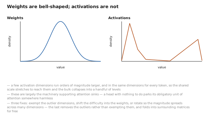
Figure 2. Weights are bell-shaped; activations are not.
Where the floor is
Four bits is comfortable. Three is noticeably degraded. Two, by direct rounding, destroys the model.
The lower range is nonetheless active, and the reason is a result from the scaling laws direction: at a fixed memory budget, a larger model quantized more aggressively often beats a smaller model quantized gently. If you have thirty-five gigabytes, a seventy-billion model at four bits generally outperforms a thirteen-billion model at sixteen. Parameters are worth more than precision, within limits, which pushes practitioners toward the largest model that will fit at whatever bit-width still works.
Pushing below three requires giving up round-to-nearest entirely. The successful approaches replace each group of weights with an index into a learned codebook of vectors, so the representation is a lookup rather than a grid — vector quantization, which exploits the fact that groups of weights are correlated and that a well-chosen set of a few hundred representative vectors covers the space far better than uniform levels do. This reaches usable quality near two bits, at the cost of a more complex and slower decode path.
And there is one thing quantization cannot fix. The KV cache is not weights, and shrinking the weights does nothing to it — so a heavily quantized model serving long conversations finds that the cache, untouched, now dominates its memory entirely. Quantizing the cache is a separate exercise with its own difficulties, keys being noticeably less tolerant than values.
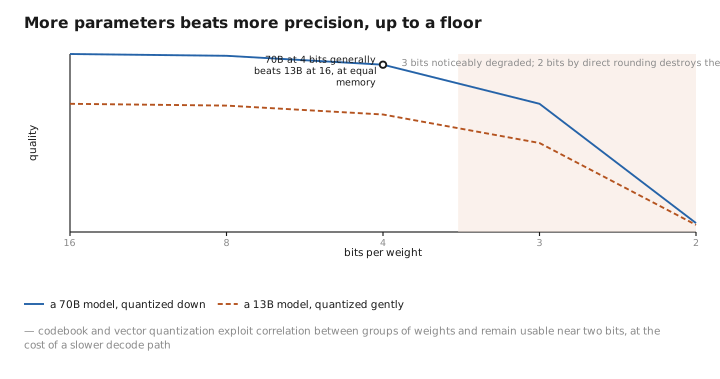
Figure 3. More parameters beats more precision, up to a floor.
What to carry forward
Quantizing a finished model is easier than quantizing one being trained, since no gradients must survive and nothing accumulates — but the damage is permanent, because there is no chance to adapt around it. The motivation is bandwidth as much as memory: generation streams every weight from memory to produce each token, so halving the weights roughly doubles the speed, while the memory saving is what decides whether the model fits on hardware at all. The mechanics are rounding to a grid with a scale per small block of values, which is nearly free at eight bits and needs help at four. That help comes from reframing the goal: the aim is not to represent the weights accurately but to preserve the layer’s outputs, which requires a calibration sample to learn what activations each layer actually sees. Two families follow — one quantizing column by column and adjusting the remaining weights to cancel the error already introduced, the other rescaling the channels that carry large activations so they land on a finer part of the grid. Quantizing the activations as well, which is what unlocks faster arithmetic rather than merely less traffic, runs into the outlier dimensions that exist to support attention sinks; the fixes exempt them, shift their scale into the weights, or rotate the representation so no single dimension is extreme. Four bits is comfortable, three is degraded, and below that requires codebooks rather than grids — and throughout, a larger model quantized harder tends to beat a smaller one quantized gently at equal memory. None of it touches the cache, which is untouched by weight compression and becomes the dominant cost once the weights have shrunk.
The figures in this article follow the shared figure key , which explains what every shape, line style and colour means.
