Before the first gradient arrives, every weight in the model has to be set to something, and the something is drawn at random. This sounds like a detail to be got out of the way, and for a long time it was treated as one. It is not. The scale of those random draws determines whether a signal survives its journey up an eighty-block tower or dies on the way; it determines whether the gradient makes it back down; and — the part that turns a numerical nicety into an economic question — it determines whether a learning rate that worked on a small model still works on a large one. That last property has a name and a construction, and it is the reason nobody tunes hyperparameters on a frontier model directly. This piece is about how the starting point is chosen and why choosing it correctly lets you do your experiments somewhere cheap.
The problem with getting the scale wrong
Take a vector, multiply it by a random matrix, multiply the result by another, and keep going. What happens to its magnitude depends entirely on how large the random entries are.
If they are slightly too large, each multiplication amplifies, and eighty amplifications compound into a number the arithmetic cannot represent. If they are slightly too small, each multiplication shrinks, and eighty shrinkages leave a signal indistinguishable from zero. The tolerance is narrow, and it narrows further with depth, because the effect is multiplicative. There is no learning to be done in either regime: the forward pass produces garbage or nothing, and the backward pass, which is subject to the same compounding, delivers a gradient that has exploded or vanished before it reaches the lower layers.
The classical fix reasons about variance. If a layer takes $n_{\text{in}}$ inputs and sums them with random weights, and we want the output to have roughly the same spread as the input, then the variance of each weight should scale as $1/n_{\text{in}}$ — because summing $n$ independent terms multiplies the variance by $n$, and we need to cancel that. Drawing weights from a distribution with
$$\text{Var}(W_{ij}) = \frac{1}{n_{\text{in}}}$$keeps activations at a stable scale layer after layer. Variants differ in whether they also account for the backward pass, which suggests $1/n_{\text{out}}$, and in how they handle the shrinkage caused by a nonlinearity that zeroes half its inputs, which suggests a factor of two. These are the schemes named after their authors, and for a plain deep network they are close to the end of the story.
For a transformer there are two amendments. Because every block adds into the residual stream and nothing subtracts, the accumulated magnitude grows with depth, so each block’s output projection is usually scaled down by a factor involving the number of layers — commonly dividing by the square root of the depth — so that the total after all blocks stays sane. And a few specific matrices are deliberately started at zero rather than at random: the second matrix of each LoRA pair, so that adaptation begins as the identity, and in some designs a learned per-block gain, so that the model begins as a stack of blocks that do nothing and switches them on as it finds a use for them.
The problem this does not solve
Standard initialization keeps a given model trainable. It does not make two models of different sizes behave alike, and that is a separate and more expensive problem.
Here is the situation anyone training a large model faces. The learning rate is the most consequential dial there is, and it has no theory that fixes it — it has to be found empirically. Finding it means training a model several times at different values and seeing which works. On a model that costs several million dollars and two months per run, that is not an experiment anybody performs. So the learning rate is tuned on a small model and reused on the large one.
Under standard initialization this transfer does not work. The optimal learning rate shifts systematically as width grows, and it shifts downward: a value that trains a small model beautifully will destabilize a wide one. Practitioners knew this and compensated with rules of thumb and with warm-up, but the compensation was folklore, and it meant every large run began with an educated guess that could not be validated until it was too late to change. A meaningful fraction of the compute spent on large models in that era went on runs that diverged.
Why does the optimum move? Because standard initialization keeps the forward activations stable at initialization and says nothing about what an update does. Consider one layer’s contribution: as width $n$ grows, an update to that layer changes its output by an amount that also scales with $n$, since more terms are being summed. A step size appropriate at width one thousand therefore produces a change several times too large at width eight thousand. The forward pass was made width-independent; the update was not.
Maximal update parameterization
The fix is to work out, for every matrix in the model, how its initialization scale and its learning rate must depend on width so that three things hold simultaneously as width grows: activations stay a constant size, the change in activations caused by one update stays a constant size, and the logits stay a constant size. Impose all three and the scalings are determined — there is essentially one answer, and it is called maximal update parameterization, usually shortened to muP.
The construction sorts the model’s matrices into three classes, and the classification is the substance of it.
Matrices whose input width is fixed and whose output width grows — the embedding table, whose input is a one-hot over a fixed vocabulary — keep an initialization variance that does not shrink with width, and a learning rate that does not shrink either.
Matrices where both dimensions grow with width — everything in the interior of the model — get the usual $1/n$ initialization variance, but their learning rate is scaled down proportionally to $1/n$. This is the crucial departure, and it is what standard practice was missing.
The output matrix, whose input width grows and whose output is a fixed vocabulary, gets its own treatment: its contribution is scaled down by a further factor of $1/n$, so that the logits entering the softmax do not grow simply because the model got wider. That downscaling can be applied in either of two equivalent places — as an initialization variance of $1/n^2$, or as a $1/n$ multiplier on the output with ordinary initialization — and implementations differ in which they choose. Doing both is a common and silent error, since it applies the correction twice.
The payoff is the property the whole exercise was for. Under muP, the optimal learning rate stops depending on width. Tune it on a model of width two hundred and fifty-six, and the same value is optimal at width eight thousand. The curve of loss against learning rate, plotted for models of many widths, lines up its minimum at the same place instead of marching leftward. The same holds for several other dials — initialization scale, output multiplier, and to a workable approximation the settings of AdamW .
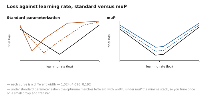
Figure 1. Loss against learning rate, standard versus muP.
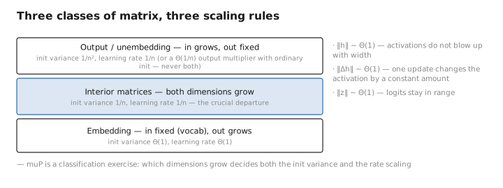
Figure 2. Three classes of matrix, three scaling rules.
A pinch of math: what is being held fixed
The reasoning is easier to trust when the target is written down. Let $n$ be the width. For each layer we want three quantities to be of order one — neither growing nor shrinking — as $n$ becomes large:
$$\|h\| \sim \Theta(1), \qquad \|\Delta h\| \sim \Theta(1), \qquad \|z\| \sim \Theta(1)$$where $h$ is a layer’s activations, $\Delta h$ is how much they move after one optimizer step, and $z$ are the final logits.
The first alone is what classical initialization achieves. The second is the new demand, and it is what forces the learning rate to scale. To see why, take a hidden matrix $W$ of shape $n \times n$ acting on an activation $h$. An update $\Delta W$ changes the output by $\Delta W \, h$, which is a sum of $n$ terms. If every entry of $\Delta W$ is of the same typical size regardless of $n$ — which is what a width-independent learning rate gives you under Adam, since Adam’s update is normalized to a size set by the learning rate alone — then that sum grows like $n$, and the second condition fails badly. Scaling the learning rate for such matrices by $1/n$ cancels it exactly.
The third condition is why the output layer is special. Its input width grows, so without intervention the logits grow too, pushing the softmax toward saturation purely as a consequence of making the model wider — an effect that has nothing to do with the model being better and everything to do with the arithmetic.
None of this requires following the derivation. The point is that the scalings are not tuned; they are the unique solution to a set of constraints, which is why the transfer works reliably rather than approximately.
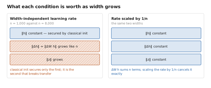
Figure 3. What each condition is worth as width grows.
What it changed in practice
The procedure this enables is now standard at scale, and it is worth stating because it explains a great deal about how large models actually get built. Sweep the hyperparameters on a family of small models — cheap, fast, many runs. Verify that the optimum has stopped moving as width increases, which is the check that the parameterization is correctly implemented. Then transfer those values to the full-size run and train once. The cost of the sweep is a small percentage of the cost of the single large run, rather than a multiple of it.
Two honest caveats. The transfer is proven for width and is much less clean for depth, where the interaction with residual connections is more delicate and where the extensions that exist are newer and less settled. And implementing muP correctly is fiddly — it touches initialization, per-parameter-group learning rates, and an output multiplier, and getting any one of them wrong silently reverts you to standard behaviour while appearing to work. The recommended check is empirical rather than theoretical: train a family of increasingly wide models, plot loss against learning rate, and confirm the minima align. If they do not, something is wired incorrectly.
What to carry forward
Weights must start somewhere, and the scale of that start decides whether a signal survives eighty multiplications on the way up and whether a gradient survives them on the way down; the classical answer sets each weight’s variance to roughly one over its number of inputs, so that summing many terms neither amplifies nor shrinks. Transformers add two amendments: scale each block’s output down according to depth, because the residual stream accumulates and never subtracts, and start certain matrices at exactly zero so that a component begins as a no-op. What classical initialization does not give you is consistency across model sizes — it stabilizes the forward pass but says nothing about the size of an update, which grows with width, so the best learning rate drifts downward as models get wider and cannot be carried from a small experiment to a large run. Maximal update parameterization fixes this by deriving, rather than tuning, how initialization and learning rate must scale for each class of matrix so that activations, the change in activations per step, and the logits all stay a constant size as width grows. The consequence is that the optimal learning rate becomes width-independent, so hyperparameters can be swept on small cheap models and transferred intact to a model a hundred times larger — which is how frontier runs are configured, since nobody can afford to tune by trial and error at that scale. The transfer is solid for width, much less settled for depth, and easy to implement incorrectly in a way that fails silently, so the practical test is to confirm that the loss-versus-learning-rate minimum stops moving as width increases.
The figures in this article follow the shared figure key , which explains what every shape, line style and colour means.
