One quantity keeps turning up across the training of language models, wearing a different job each time. It is the imitation metric in distillation , the leash in DPO and in reinforcement learning from human feedback, one of the damage measures in ablation , and the term that training actually minimizes once cross-entropy is decomposed. Four unrelated-looking uses, one formula. It is worth understanding on its own terms rather than meeting it four times as a piece of notation, particularly because it has a property that surprises everyone the first time — it is not symmetric, and which way round you write it changes what you are asking for. This piece is about what the quantity measures, why the asymmetry is a feature rather than a defect, and how to tell which direction you want.
Measuring a gap between beliefs
Suppose two distributions over the same set of outcomes: $q$, which describes what actually happens, and $p$, which describes what you believe. How far apart are they?
The naive answers all fail. Comparing the most likely outcome under each throws away everything else. Summing the absolute differences treats a gap between 0.50 and 0.51 as equal in importance to a gap between 0.001 and 0.011 — but the second is a tenfold error and the first is a rounding difference. What is wanted is a comparison of ratios, and one that weights each outcome by how often it actually occurs.
The article on cross-entropy supplies the route. Surprise at an outcome of probability $p_i$ is $-\log p_i$; the average surprise you actually experience, believing $p$ while reality follows $q$, is $-\sum_i q_i \log p_i$; and the least you could possibly experience, if your beliefs were exactly right, is $-\sum_i q_i \log q_i$. The gap between the two is the waste attributable to being wrong:
$$D_{\text{KL}}(q \,\|\, p) \;=\; \sum_i q_i \log \frac{q_i}{p_i}$$That is the Kullback–Leibler divergence, and the interpretation is exact rather than metaphorical. It is the number of extra bits per outcome you pay by encoding data from $q$ using a code designed for $p$. Zero when the two distributions coincide, positive otherwise, and never negative — a fact that follows from the concavity of the logarithm and can be taken on trust.
Three properties are worth holding onto. It compares log-ratios, so it cares about relative rather than absolute differences. It weights each outcome by $q_i$, the probability of actually being there — outcomes that never occur under $q$ contribute nothing regardless of how wrong you are about them. And it is unbounded: if $q$ puts real probability on something $p$ considers impossible, the ratio blows up and the divergence is infinite.
Why it is not a distance
Swap the arguments and you get a different number. $D_{\text{KL}}(q \| p) \neq D_{\text{KL}}(p \| q)$, and often the two are wildly different. It also fails the triangle inequality. It is therefore not a metric, which is why the literature is careful to call it a divergence.
This looks like a defect and is in fact the most useful thing about it, because the two directions ask genuinely different questions.
The forward direction, $D_{\text{KL}}(q \| p)$, averages over where $q$ has mass. Every outcome that really happens contributes, weighted by how often. The penalty for putting too little probability on something real is severe — the log-ratio grows without bound as $p_i \to 0$ — while putting probability on something that never happens costs nothing, since those terms are weighted by $q_i = 0$. Minimizing in this direction therefore produces a $p$ that covers everything $q$ does. Faced with a $q$ that has two separate peaks and a $p$ that can only manage one, the forward direction will smear $p$ across both, including the empty valley between them, rather than leave either peak uncovered. It is mass-covering, and its failure mode is a model that hedges, spreading probability over things that do not occur.
The reverse direction, $D_{\text{KL}}(p \| q)$, averages over where your own distribution has mass. Now the terms are weighted by $p_i$, so you are only penalized where you put probability. Placing mass where $q$ has none is catastrophic; declining to place mass somewhere $q$ has plenty costs nothing at all. Minimizing in this direction produces a $p$ that concentrates on one region and stays safely inside the support of $q$. Given the same two-peaked $q$, it picks a peak and commits. It is mode-seeking, and its failure mode is a model that ignores most of the possibilities.
The picture to keep is a blanket. The forward direction insists the blanket cover everything, and will accept a thin blanket over empty floor to manage it. The reverse direction insists the blanket only touch the bed, and will accept covering half the bed to guarantee it.
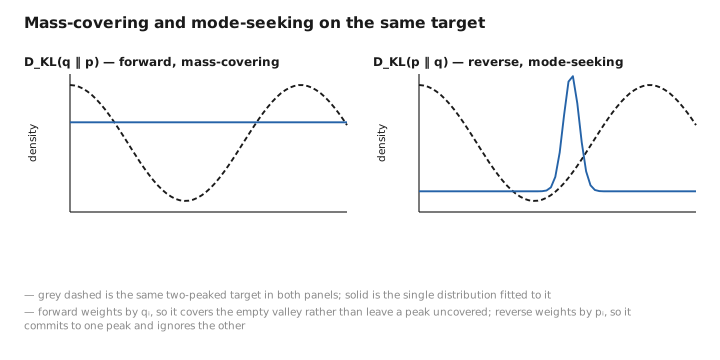
Figure 1. Mass-covering and mode-seeking on the same target.
Which direction each use wants
With that distinction, the four appearances sort themselves out.
Ordinary training uses the forward direction, though it is rarely written that way. Minimizing cross-entropy against the empirical data is minimizing $D_{\text{KL}}(\text{data} \| \text{model})$, since the entropy of the data is a constant the model cannot affect. This is why language models are mass-covering — they assign some probability to nearly everything, and will happily hedge. It is the right choice for a model meant to represent the full range of what text can be, and it is also why sampling directly from a model gives less impressive text than truncated decoding does. The training objective asked for coverage; the reader wanted commitment.
Distillation uses the forward direction with the teacher as $q$. The point is precisely to inherit the teacher’s full distribution, including the relative plausibility of the wrong answers, so mass-covering is exactly what is wanted.
The RL leash uses the reverse direction, with the policy as $p$ and the starting model as $q$ — and here the mode-seeking property is doing deliberate work. The penalty is enormous for the policy putting probability anywhere the reference model considered near-impossible, which is exactly the constraint desired: do not wander off into strange regions of language where the reward model’s judgement cannot be trusted. It is indifferent to the policy narrowing, which is also correct, since narrowing onto good behaviour is the entire point of the exercise. A forward-direction leash would have insisted the policy keep hedging like the base model, which would defeat the purpose.
DPO does not compute a divergence at all, but its implicit reward is $\beta \log(\pi/\pi_{\text{ref}})$ — the log-ratio that sits inside the sum. The constraint is built into the shape of the reward rather than added as a term, which is what that article means by the leash being structural.
Ablation uses it as a symmetric-in-spirit damage measure, asking how much the whole output distribution moved when a component was removed. Here neither direction is obviously right, which is why practitioners often report the symmetrized version instead.
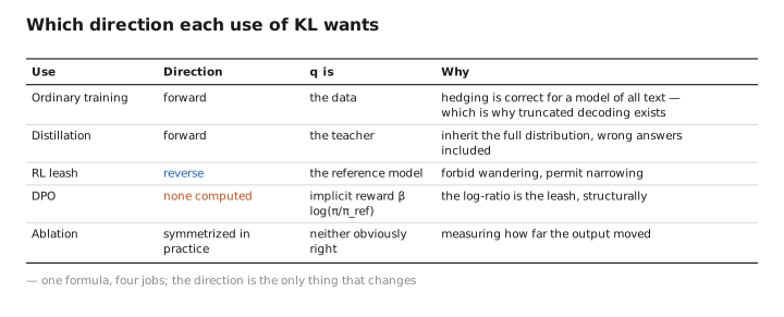
Figure 2. Which direction each use of KL wants.
Estimating it in practice
Two practical points, because the formula as written is often not what gets computed.
Over a full vocabulary the sum is exact and cheap, since the model gives all the probabilities. This is the case in distillation and in ablation, and there is nothing to approximate.
Over sequences it is intractable, because the sum runs over every string that could ever be generated. The RL leash is in this situation, and the usual approach is to estimate from samples: draw sequences from the policy and average $\log(\pi/\pi_{\text{ref}})$ over them. This is unbiased but noisy, and it can go negative on any particular batch even though the true value cannot, which is disconcerting when it appears on a dashboard. A better estimator adds a correction term that is zero in expectation but cancels much of the variance, giving something that stays non-negative sample by sample. It is a small implementation detail with a visible effect on how stable a training run looks.
The other point concerns the infinity. If the model assigns exactly zero to something the reference assigns real probability, the divergence is infinite and the gradient is meaningless. In practice a softmax never outputs exactly zero, so this rarely bites during training — but it bites immediately if the distribution has been truncated before comparison, which is a genuine trap when evaluating models under their sampling settings rather than raw.
What to carry forward
KL divergence measures the gap between two distributions as the extra bits per outcome you pay for believing $p$ when reality follows $q$ — a comparison of log-ratios, weighted by how often each outcome actually occurs, zero when the distributions agree and never negative. It is not symmetric, and the asymmetry is the point. The forward direction, averaging over where the truth has mass, punishes leaving anything real uncovered and ignores probability spent on things that never happen, so it is mass-covering and produces models that hedge; the reverse direction, averaging over where your own distribution has mass, punishes only where you have committed, so it is mode-seeking and produces models that pick a region and stay inside it. Ordinary language-model training and distillation both use the forward direction, which is why models hedge by default and why truncated decoding is needed to get committed text out of them. The reinforcement-learning leash uses the reverse direction deliberately, because the goal is to forbid wandering into regions the reference model considered implausible while permitting the policy to narrow. Over a vocabulary the sum is exact and cheap; over sequences it must be estimated from samples, where a variance-reduced estimator avoids the disconcerting negative values a naive one produces. And the quantity is unbounded, going infinite the moment one distribution assigns real probability to something the other rules out entirely.
The figures in this article follow the shared figure key , which explains what every shape, line style and colour means.
