The learning rate is usually introduced as a number: one small constant, multiplied into every gradient and then left alone. Almost no large model has ever been trained that way. In practice it is a function of the step count — near zero for the opening few thousand steps, rising to a peak, then falling for the rest of the run — and the shape of that function is treated as somewhere between a solved problem and a superstition. It is neither. The opening ramp exists for a specific and slightly embarrassing reason to do with the optimizer’s own bookkeeping, and the conventional curve imposes a constraint so awkward that an entire alternative arrangement was invented to escape it. This piece is about why the rate has to move at all, what the two halves of the schedule are separately doing, and what the standard shape quietly costs.
One step size cannot serve a whole run
The rate has to move because the run is not one problem. It is at least two, and they want opposite things.
Early on, almost any direction is downhill. The weights are random draws, the model is producing noise, and the gradients arriving from successive batches are large and in broad agreement, because every example is objecting to the same gross errors — the output distribution is flat where it ought to be sharply peaked, and correcting that is a consensus project. There is little disagreement to average away and a great deal of ground to cover, so a long step is valuable, though the optimizer’s own running estimates have barely been assembled.
Late on, what remains is disagreement. The obvious structure has been absorbed, the gradients are small, and consecutive batches now argue about what to do next, since what is left to learn is precisely the part on which examples do not agree. A long step here covers no ground. It responds at full volume to whichever few hundred thousand tokens happened to arrive, then does it again in the opposite direction.
A single number is either too timid for the first regime or too loud for the second, and the schedule is the admission that no compromise value is good in either.
The peak value has no theory behind it either, and two couplings catch people out. It depends on the batch size , since a cleaner gradient supports a bolder step, and the working rule is to scale the rate with the square root of the batch — approximate, and valid only up to a ceiling set by the curvature of the landscape rather than by the data. It depends also on the width of the model, which is why a rate tuned on a small proxy does not transfer under ordinary initialization ; making it transfer is exactly what muP-style parameterization is for.
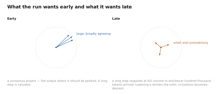
Figure 1. What the run wants early and what it wants late.
Warm-up buys time for a badly estimated denominator
The folklore explanation for warm-up is that the model is fragile at the start and should be handled gently. That is not wrong. It is also not the mechanism.
An adaptive optimizer such as AdamW does not apply the gradient directly. It divides the smoothed gradient by a running estimate of recent gradient magnitude, so that every parameter steps in units of its own typical behaviour. The denominator is the whole trick. At step ten it is an average over ten samples, and an estimate built from that little data is not merely imprecise; it is occasionally wildly wrong in the dangerous direction, too small. A confident step divided by a badly underestimated denominator is an enormous step taken on no evidence. That is how a run dies in its first thousand steps, quietly, leaving a curve that looks as though learning never started rather than one that broke.
Ramping the rate from near zero over a few thousand steps buys time for the estimate to accumulate enough samples to be trusted, at the cost of steps deliberately smaller than would have worked. It is insurance, paid for in data.
This is also why bias correction exists, and the two are easily confused. The running averages start at zero, so for the opening steps they are dragged toward zero and understate both the gradient and its magnitude; the correction inflates them back to honest size. That fixes the bias. It does nothing about the variance, which is what warm-up is for. A correctly bias-corrected optimizer with no warm-up still takes a catastrophic step the first time its denominator comes out small, so anyone who removes the ramp on the grounds that bias correction already handles the opening steps will meet a loss spike within the hour.
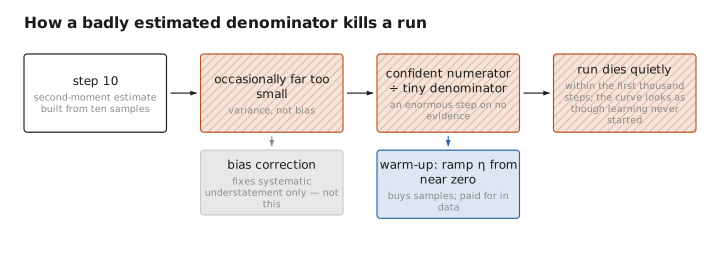
Figure 2. How a badly estimated denominator kills a run.
Decay converts bouncing into settling
What the decay buys is best described geometrically. Every step of gradient descent is the true descent direction plus a noise term inherited from sampling a finite batch, and both scale with the rate. At a large rate the noise is large enough that the parameters circulate around the bottom of a region at a fixed radius rather than descending into it, like tea leaves in a cup still being stirred. Lowering the rate shrinks the radius. Circulation becomes descent, and the loss drops for reasons that have nothing to do with new information and everything to do with the parameters finally being allowed to arrive.
That is the honest account of the sharp late-run improvement people see when the rate anneals. It is not the model suddenly learning. It is the model stopping.
The conventional curve is cosine decay, from the peak down to a tenth of it or to zero across the whole run, and its standing deserves scrutiny. Linear decay works about as well; inverse-square-root nearly as well; at matched budgets the gaps between them are small enough to be swamped by other choices. What matters is that the rate spends a long stretch high and finishes very low, not the route between. There is no derivation of the shape. Cosine is a convention that works, kept because it is what everyone else uses, and treating it as an optimum is the same error as treating any long-standing default as a result.
Decaying the rate also weakens the weight decay, and almost nobody accounts for it. Decoupled decay pulls every weight toward zero by a fraction proportional to the current rate, so as the rate falls the tether slackens in exact proportion, and by the end of a cosine run the regularization operates at a tenth of its nominal strength or less. The schedule anneals two things while appearing to anneal one.
A pinch of math: where the total step count hides
Write $\eta_t$ for the rate at step $t$. The warm-up is a straight line, $\eta_t = \eta_{\max}\, t / T_w$ for $t < T_w$, and the cosine phase that follows is
$$\eta_t = \eta_{\min} + \tfrac{1}{2}(\eta_{\max}-\eta_{\min})\left(1 + \cos\left(\frac{\pi t}{T}\right)\right)$$At $t = 0$ the cosine is $1$ and the rate is $\eta_{\max}$; at $t = T$ it is $-1$ and the rate is $\eta_{\min}$. The derivative is near zero at both ends and largest in between, so the curve lingers at the top, falls quickly through the middle, and lingers again at the bottom — the property usually credited for its success.
The load-bearing symbol is $T$. It is not a stopping condition applied to a curve defined independently of it; it sits inside the argument of the cosine, so the rate at step fifty thousand of a run planned for one hundred thousand steps is not the rate at step fifty thousand of a run planned for two hundred thousand. Doubling the intended length does not extend the schedule. It redraws every point on it. That is the whole practical problem in one line: to evaluate $\eta_t$ at all, you must already have decided when the run ends.
The plan is fixed before the run begins
Because the total step count lives inside the formula, a cosine run is one indivisible object. It cannot be extended, since extending it would have required a different curve from the start, and cannot be usefully resumed at a longer horizon for the same reason. Every checkpoint before the end is not a finished model trained for less time but a model caught mid-anneal, still circulating at a rate chosen for a run that has not finished, and therefore worse than a model properly cooled down at that budget. For anyone who wanted a curve of loss against training duration, that is expensive: every point on it is a separate run.
The fix is to separate the high phase from the descent. Hold the rate flat for the great majority of the run, then decay it sharply at the very end over a few percent of the steps. This constant-then-cooldown arrangement reaches loss comparable to a well-tuned cosine and removes the dependence on knowing the total in advance, because a flat phase is indifferent to when it stops. Train as long as the budget allows, stop, cool down over a short tail, and the result is a finished model rather than an interrupted one. This is what makes the scaling-law practice of reading many points off one run possible, and a fair illustration of how far a scheduling convention can constrain the experiments people are able to imagine.
What no schedule does is react to the run. It is an open-loop plan, computed from the step index and nothing else, indifferent to whether the loss is falling nicely, has flattened, or has just spiked by two nats. The optimizer adapts per parameter; the global rate does not adapt at all. Alternatives exist — rates derived from gradient statistics, methods that dispense with a horizon, controllers that watch the loss — and they have not displaced the fixed schedule despite being competitive in narrow comparisons. The reason is not that they fail. It is that a fixed schedule is predictable, so it can be planned in advance and blamed or exonerated afterwards, and predictability is worth a great deal when a run costs millions and cannot be repeated.
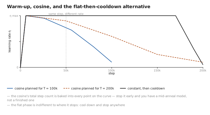
Figure 3. Warm-up, cosine, and the flat-then-cooldown alternative.
What to carry forward
A learning rate is a function, not a constant, because a run makes contradictory demands: early, the model is producing noise, gradients are large and in broad agreement, and long steps are safe; late, gradients are small and mutually contradictory, and the useful move is to settle. Warm-up handles the opening, for a sharper reason than fragility — an adaptive optimizer divides by a running estimate of gradient magnitude, built from almost no samples at first, and a confident step divided by a badly underestimated denominator is how a run dies in its first thousand steps; ramping from near zero buys time for it to be trusted, a different complaint from the systematic understatement bias correction fixes, and conflating the two loses runs. Decay converts circulation into descent, since a high rate keeps the parameters orbiting a basin rather than entering it; the late fall in loss is arrival, not insight. Cosine is the default, its shape matters less than its reputation, and no derivation stands behind it. Its real cost is that the total step count sits inside the formula: the run cannot be extended or resumed, and every intermediate checkpoint is mid-anneal rather than finished, which is why holding the rate flat and cooling sharply at the end has displaced it wherever the stopping point is not yet chosen. Two couplings stay easy to miss — the peak scales roughly with the square root of the batch and will not cross model widths without a parameterization built for it, and decoupled weight decay is proportional to the current rate, so annealing one anneals the other. And none of it adapts. The schedule is a plan written before the first step, indifferent to what the loss then does, kept because it is predictable rather than because it is right.
The figures in this article follow the shared figure key , which explains what every shape, line style and colour means.
