The loss curves that appear in technical reports are smooth. They descend, they flatten, and they suggest that training a large language model is a matter of starting the machinery and waiting. The curves kept by the people running those jobs look different. Somewhere around step forty thousand, with nothing changed in the configuration, the loss jumps — not drifts, jumps — by a whole nat or two inside a handful of steps, and then does one of three things: claws its way back over a few thousand steps, settles permanently above the trajectory it left, or keeps rising until the model emits one token forever. This is a loss spike, and it is why a frontier run is watched on a rota rather than left alone over a weekend. This piece is about what happens when a run falls over, why the proposed causes are still argued about, and what the available defences cost.
What a spike looks like from the logs
The defining feature is the timescale. A run whose loss has descended for tens of thousands of steps, smoothly enough to fit a scaling law through, moves one or two nats in five or ten steps. On a plot of the whole run it is a vertical line. Zoom in and the gradient norm has almost always gone first, one step at ten or a hundred times its recent value, with the loss following immediately, because the step that norm produced is already in the weights.
What follows is not one behaviour but three. Sometimes it recovers unaided, descending more steeply and rejoining its old trajectory within a few thousand steps. Sometimes it recovers most of the way and stops, tracking parallel to where it was but permanently above it, and the run finishes worse than intended. And sometimes it does not recover: the loss climbs to what guessing would give, or ceases to be a number, and what remains puts all its mass on one token regardless of input.
The reason this is studied rather than shrugged at is arithmetic. A large pretraining run occupies thousands of accelerators for weeks, costs millions of dollars, and cannot be repeated with a different seed to see whether the trouble goes away. There is one run. If it spikes at the halfway mark and lands in the second outcome, the money has been spent and the model that emerges is not the one budgeted for.
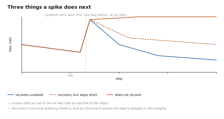
Figure 1. Three things a spike does next.
Small models are hard to destabilize and large ones are not
The first thing any explanation has to account for is the size dependence, and it is stark. Small models are remarkably difficult to break. Set the learning rate too high and a model of a few hundred million parameters merely trains badly, converging to a worse loss without the characteristic discontinuity; feed it a corrupted batch and it absorbs it. The same configuration at ten times the parameters will spike, sometimes repeatedly, sometimes fatally.
This is what makes spikes a property of scale rather than a defect in anyone’s code. A bug would show at every size and be findable by ordinary means. Instead, instability appears gradually as width and depth grow, in a configuration validated cheaply and never doubted. The validation was honest; the transfer was the problem. Whatever the mechanism, its severity must grow with the model, which rules out a good many otherwise plausible stories.
Four mechanisms wear the same symptom
The specific culprit is still argued over, and groups running comparable models have reported different dominant causes. What is not argued over is the shape of the failure: something develops an unusually large magnitude, one step is taken far too big, and the resulting weights are either recoverable or not. Four candidates produce that shape, they are not exclusive, and the argument persists because a spike leaves too little evidence to say which it was.
The leading candidate is attention logit growth. Query-key dot products are constrained by nothing. Over a long run some heads acquire larger projection norms, the scores grow with them, and the softmax saturates — one weight goes to essentially one, the rest to essentially zero. A saturated softmax has almost no gradient, so the head stops receiving a corrective signal and the drift that caused the saturation goes unopposed. That is the self-reinforcing part. The output, meanwhile, has become a near one-hot selection of one position’s value vector, and selection is discontinuous: a small change in the projections moves which position wins, and the output jumps by the whole difference between two value vectors. Untrainable and violently sensitive at once. It worsens with width, since a dot product over more dimensions sums more terms and saturation arrives sooner.
The second is the optimizer’s own memory. An adaptive optimizer divides each step by a slow-moving estimate of that parameter’s recent gradient magnitude, slow by design so the sense of scale stays steady. That is the wrong property when a batch delivers a gradient a hundred times larger than anything recent: the denominator still reflects the old magnitudes, the numerator the new one, and the step is enormous. The estimate catches up within a few dozen steps, which is why the anomaly ends quickly in the log, but the damage was in the weights first. This is why practitioners shorten that memory for large models by lowering the second-moment decay constant. A shorter memory still has a memory. It is a mitigation, not a cure.
The third is numerical range. A sixteen-bit format with five exponent bits leaves little headroom above ordinary activation magnitudes, and an overflow anywhere produces an infinity that propagates through the backward pass into the gradient, into the optimizer state, and from there into every weight it touches. One bad value poisons the model in a single update. The shift to mixed-precision formats with the exponent range of single precision removed this class almost entirely and left the others as they were, which is the most useful evidence in the subject: several distinct mechanisms were plainly wearing one symptom.
The fourth, and the least satisfying, is the data. A single pathological batch can produce a gradient unlike anything the run has seen: ten thousand repetitions of one token, binary that survived the filters, a script the tokenizer handles badly. This is real, it is the easiest of the four to fix, and it explains fewer spikes than people hope. Careful data curation removes the worst offenders, and runs still spike on batches later inspected and found unremarkable.
A pinch of math: what growing logits buy on both sides
Write the attention weights over a row of scores $z_1 \ldots z_n$ in the usual way,
$$p_i = \frac{e^{z_i}}{\sum_j e^{z_j}}$$with the head’s output the weighted sum $o = \sum_i p_i v_i$. Two derivatives matter, and they move in opposite directions as the scores grow.
The first is how much a weight responds to a score:
$$\frac{\partial p_i}{\partial z_i} = p_i(1 - p_i), \qquad \frac{\partial p_i}{\partial z_j} = -\,p_i p_j \quad (j \neq i)$$Every one of those terms collapses toward zero once any single $p_i$ approaches one: the diagonal term is maximized at $p_i = 1/2$ and vanishes at both extremes, and the off-diagonal terms are products of a number near one with numbers near zero. A saturated softmax has almost no derivative anywhere, so whatever gradient arrives from above is multiplied by something near zero and never reaches the projections that produced the scores.
The second is how much the output responds to which score is largest. As $p$ becomes one-hot on index $a$, the output approaches $v_a$. Move the largest score from $a$ to $b$ and the output moves by $v_a - v_b$ — a whole difference between two value vectors, of order one, with no tendency to shrink as the logits grow, since nothing has trained those vectors to resemble each other.
Growing logits therefore buy a vanishing gradient and a rising discontinuity at once, in the same head. The smooth stand-in for the maximum has quietly become the maximum: flat nearly everywhere, with a cliff. That combination is the mechanism.
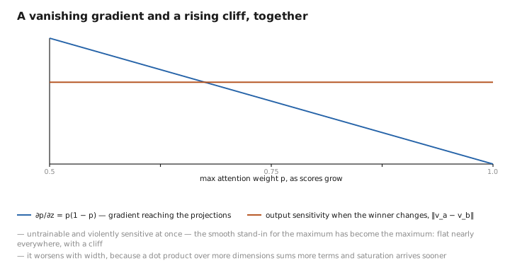
Figure 2. A vanishing gradient and a rising cliff, together.
Every mitigation charges something for its help
None of the defences in use is free, and the honest way to present them is with the bill attached.
Gradient clipping by global norm is nearly universal and almost free. Compute the norm of the whole gradient and, if it exceeds a threshold, rescale down to that threshold before the optimizer sees it, turning a catastrophic step into a merely large one. It also changes the problem being solved: on any step where it fires, the direction is preserved but the magnitude was chosen by an engineer, not by the loss surface.
Normalizing the queries and keys before the dot product attacks the first mechanism directly, capping how large a score can become whatever the projections do. It costs two small normalization operations per head per token and removes a degree of freedom, since a head can no longer express confidence through score magnitude alone.
An auxiliary loss on the softmax normalizer — penalizing the logarithm of the denominator, so logits are pushed back whenever they drift upward — works, and adds a term to the objective that nobody wanted. Its coefficient is one more thing to tune, and it trades a little of the primary loss for stability.
Lowering the learning rate, or the second-moment constant, or both is the mid-run response of last resort, and it works by making everything slower. A schedule reduced for safety reaches a worse loss for the same compute, and since the counterfactual was never run, what was surrendered cannot be measured.
The brute-force operational answer is what large runs actually do. Checkpoint every few hundred steps; when the monitoring catches a spike, stop, rewind a few thousand steps, skip the batches that were in flight, and resume. It is unsatisfying, it costs storage and the discarded steps, and it works often enough to be standard procedure rather than a fallback.
What is not available is prediction. No signal reliably says a spike is coming before the gradient norm moves, there is no agreement on which mechanism dominates at a given scale, and no theory says whether a recovered run ends where one that never spiked would have. Practice here is a long way ahead of understanding.
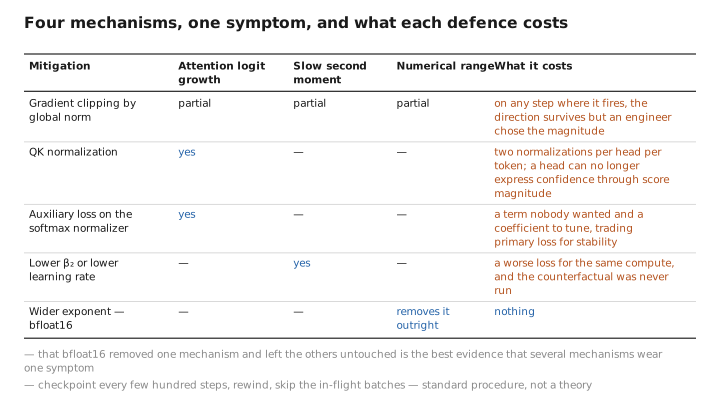
Figure 3. Four mechanisms, one symptom, and what each defence costs.
What to carry forward
A large run can descend smoothly for tens of thousands of steps and then lose one or two nats in five, after which it either climbs back, settles permanently at a worse level, or degenerates into a model that emits one token forever. All three occur, and since the run cannot be repeated, the second outcome is as expensive as the third. This is a phenomenon of scale rather than a defect: small models resist destabilization, and a configuration validated at a smaller size will spike at ten times that size, so the mechanism must involve magnitudes that grow with the model. Four mechanisms fit, and they are not exclusive. Query-key dot products drift upward until the softmax saturates, at which point the head has almost no gradient while its output is a near one-hot selection that swings discontinuously. An adaptive optimizer divides its step by a slow estimate of gradient scale, so a gradient far above recent history produces a step far above any intended size, and the estimate corrects itself only after the damage is done. A narrow exponent range permits an overflow whose infinity propagates into every parameter; a wider-range format removed that class and left the rest untouched. A pathological batch can do it too, less often than hoped. The defences all charge something: clipping changes the problem being solved whenever it fires, normalizing queries and keys costs a degree of freedom, a penalty on the softmax normalizer adds a term nobody wanted, and a lowered learning rate buys stability with loss. What large runs rely on is frequent checkpointing and rewinding on a spike, which is not a theory of anything. Nothing predicts a spike before the gradient norm moves, and nothing says whether a recovered run ends where an untroubled one would have.
The figures in this article follow the shared figure key , which explains what every shape, line style and colour means.
