A transformer does not care what its inputs mean. It consumes a sequence of vectors and produces a sequence of vectors, and nothing in attention or the feed-forward layers makes any reference to language. The embedding table is the only component that assumes its inputs are tokens, and it is a lookup rather than a computation. Which means the path to a model that sees is narrower than it looks: if you can turn an image into a sequence of vectors that live in the same space as token embeddings, the rest of the machinery will process it without modification. The interesting question is not whether this works — it plainly does — but what it costs, what gets lost, and why a model that can describe a photograph in detail will confidently misread a clock face. This piece is about the join between a vision system and a language model, and what remains awkward about it.
Images as sequences
The first step is to make an image into something sequence-shaped. The standard answer is to cut it into a grid of square patches — typically fourteen or sixteen pixels on a side — flatten each into a vector, and treat the resulting list as tokens. A 224-pixel image at 14-pixel patches becomes 256 patches, which is a sequence length a transformer handles comfortably.
This is tokenization with a different substrate, and it inherits the same character: a fixed, non-learned segmentation that decides what the model can distinguish. It also inherits the same failure mode. A patch grid imposes a resolution floor, and detail finer than a patch is averaged away before the model sees anything. Small text, thin lines, the position of a clock’s minute hand relative to its tick marks — these are sub-patch details, and a model that misreads them is not being careless. It received an average.
The quadratic cost of attention makes this hard to fix by simply using smaller patches, since halving the patch size quadruples the sequence length. The practical response has been to process a high-resolution image as several crops — a downscaled view of the whole plus a grid of full-resolution tiles — and let the model combine them. This is why the token cost of an image in current systems scales with its dimensions rather than being fixed, and why a dense screenshot can consume several thousand tokens.
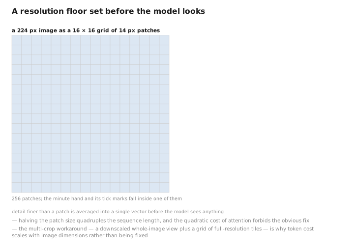
Figure 1. A resolution floor set before the model looks.
Three ways to join the two halves
Given patch vectors, the question is how they meet the language model. Three arrangements have been used, and the field has converged fairly decisively.
Cross-attention. Leave the language model’s own sequence alone and add extra attention layers that let text positions attend to image features held separately. The image never enters the text sequence, so it costs no context length, and the language model’s original weights can be frozen while only the new layers train. This was the early approach and it works. Its drawback is architectural surgery: the language model must be modified, which means the arrangement does not travel to a new base model without redoing it.
Projection into the sequence. Run the image through a vision encoder, pass the resulting patch features through a small trained network — often just one or two matrices — that maps them into the language model’s embedding space, and insert them into the token sequence as if they were tokens. Nothing about the language model changes. From its point of view it is reading a sequence of vectors, some of which happen to have come from somewhere other than the embedding table.
Resampling. A middle option that uses a small set of learned queries to attend over the patch features and produce a fixed number of output vectors, compressing an arbitrary number of patches into, say, sixty-four. This bounds the context cost regardless of image size, at the price of discarding detail through the bottleneck.
The second has won, for a reason worth naming: it requires no modification to the language model at all, so any improvement to the underlying model is inherited immediately, and the connecting network is small enough to train cheaply. The elegance is that the “projector” is doing something conceptually trivial — a change of coordinates — and the heavy lifting is done by two components that were trained separately for other purposes.
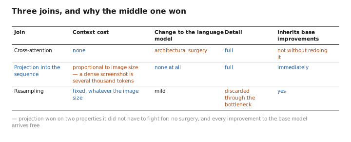
Figure 2. Three joins, and why the middle one won.
Why the vision encoder is usually contrastive
The vision half is generally not trained from scratch alongside the language model. It is a pretrained encoder, and the pretraining objective that dominates is contrastive — the same arrangement described under retrieval embeddings , applied across modalities.
Take a very large collection of images paired with their captions. Encode each image and each caption, and train so that an image is closer to its own caption than to any other caption in the batch. Both encoders learn in tandem, and what results is an image encoder whose outputs are organized by semantic content — because the only thing that predicts a caption is what the image is about.
This matters for the join. A vision encoder trained to classify images into a thousand categories learns features useful for those categories. A contrastively trained one has been shaped by natural language descriptions of unrestricted variety, so its representation is already aligned with the kinds of distinction language makes. Bolting it to a language model is a shorter journey. The projector’s job is a coordinate change rather than a translation.
The connection also runs the other way: diffusion models that generate images from text use the same kind of jointly-trained encoder to condition on a prompt, which is why the same family of models underpins both understanding and generation.
A pinch of math: the training is the ordinary one
The surprising part of the whole arrangement is how little the objective changes.
Write the input sequence as a mixture of embedded tokens and projected patches:
$$h_0 = \big[\, e(t_1), \ldots, e(t_k), \; P(v_1), \ldots, P(v_m), \; e(t_{k+1}), \ldots \,\big]$$where $e$ is the embedding lookup, $v_j$ are patch features from the vision encoder, and $P$ is the projector. The model then runs exactly as before, and the loss is exactly as before — cross-entropy on the next text token:
$$\mathcal{L} = -\sum_{t \in \text{text}} \log p_\theta(x_t \mid x_{Training proceeds in two stages that follow directly from this. First, freeze both the vision encoder and the language model and train only the projector, on a large set of image-caption pairs — this aligns the coordinate systems cheaply, with very few parameters moving. Then unfreeze the language model, and often the vision encoder, and train on richer instruction-following data involving images. The first stage teaches the two halves to speak; the second teaches the combination to be useful.
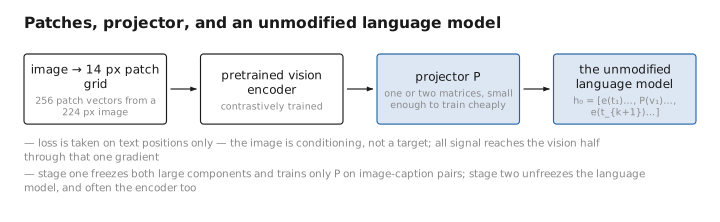
Figure 3. Patches, projector, and an unmodified language model.
What remains awkward
Four honest limitations, all of which follow from the construction rather than from insufficient scale.
Fine detail is lost before the model sees it, for the patching reason above. Clock faces, small text, precise counts of many similar objects, exact spatial relationships — the model is working from averaged tiles, and no amount of reasoning recovers information that was discarded at the input.
Spatial reasoning is weak. Patches arrive with position encodings, so the model knows where each was, but the encoding is the same kind of learned positional information used for text, and relationships like above, behind, or aligned with have to be reconstructed from it rather than being available directly. Performance on tasks requiring precise geometry is markedly worse than on tasks requiring recognition.
Attention is asymmetric between the modalities. Language dominates, because the language model is far larger, was trained on far more data, and supplies the only loss. A vision-language model asked a question whose answer is in the image but which has a strong linguistic prior will often produce the prior — answering what is usually true rather than what is shown. This is the mechanism behind a large share of visual hallucination.
The image is not tokenized in any interpretable way. A text token corresponds to a piece of text you can point at. A patch vector corresponds to a square of pixels, but its content after the vision encoder is an opaque feature, so the usual interpretability tools — sparse autoencoders , ablation — have much less purchase on the visual half.
The direction of travel is toward removing the join altogether — training a single model on interleaved text, images, audio, and video from the start, with objectives on every modality rather than only on text. That is more expensive and conceptually cleaner, and it is what the largest current systems increasingly do. The two-part construction described here remains the standard way to give an existing language model eyes without retraining it, and it will remain so for as long as the language half is the expensive part.
What to carry forward
A transformer processes sequences of vectors and does not care where they came from, so making a language model see requires only turning an image into vectors that live in the same space. Images are cut into a grid of patches, which is tokenization with a different substrate and inherits the same character — a fixed segmentation that sets a resolution floor, below which detail is averaged away before the model receives anything. Of the ways to join the halves, the one that won is the simplest: run the image through a pretrained vision encoder, pass the patch features through a small projector into the embedding space, and insert them into the token sequence, leaving the language model entirely unmodified so that any improvement to it is inherited for free. The vision encoder is typically trained contrastively against captions, which organizes its representation around the distinctions language makes and shortens the projector’s job to a change of coordinates. The training objective is unchanged — cross-entropy on the next text token, with no loss on image positions at all, so the image is conditioning rather than a target and all signal reaches the vision side by backpropagation through the projector; the standard recipe freezes both large components and trains only the projector first, then unfreezes for instruction data. What remains awkward follows from the construction: fine detail is discarded at the patch grid and cannot be reasoned back, spatial relationships must be reconstructed from position encodings rather than being directly available, and the language half dominates so strongly that a strong linguistic prior will often override what the image actually shows — which is where a large share of visual hallucination comes from.
The figures in this article follow the shared figure key , which explains what every shape, line style and colour means.
