Every block in a transformer is preceded by a small operation that rescales its input, and it is the least glamorous thing in the architecture. It computes no features, stores no knowledge, and would be omitted from any diagram drawn on a napkin. It is also the difference between a model that trains and one that does not. The residual stream grows as it rises, because every block adds and nothing subtracts; a block trained to read a signal of one typical size will misbehave when handed one ten times larger; and the gradient inherits every one of those distortions on the way back down. This piece is about the operation that keeps the numbers in range, the variant that discarded half of it and lost nothing, and the placement decision that mattered more than either.
The problem with a signal that drifts
Consider what a block actually needs from its input. Its weights were set during training under some particular distribution of incoming values, and everything about its behaviour — which activations saturate, how large its outputs are, how sensitive it is to a small change — depends on that distribution holding. If the input arrives at three times the expected magnitude, the block’s contribution is roughly three times too large, that contribution is added to the stream, and the next block receives something further out of range still.
Now stack eighty of these. Small drifts compound multiplicatively, and the top of the tower ends up operating in a regime the bottom never saw. Worse, the drift moves during training: as the early layers’ weights change, the distribution they emit changes, and every later layer finds that the input it had adapted to has shifted underneath it. Each layer is chasing a target that the layers below keep moving. The condition has a name — internal covariate shift — and while the original diagnosis has been argued over ever since, the practical fact is not in dispute. Unnormalized deep networks are difficult to train, need tiny learning rates, and are exquisitely sensitive to initialization.
The gradient suffers symmetrically. A backward pass through a layer scales the gradient by something related to that layer’s magnitudes, and eighty such scalings compound into the same vanishing or exploding problem that residual connections were introduced to solve. Residuals fix the path; they do not fix the scale.
The fix: standardize before every block
The remedy is to insert, before each block, an operation that puts its input into a known state regardless of what arrived. Layer normalization does this by working across the features of a single token: compute the mean and standard deviation of that token’s vector, subtract the mean, divide by the standard deviation.
$$\hat{x} = \frac{x - \mu}{\sqrt{\sigma^2 + \epsilon}}, \qquad \mu = \frac{1}{d}\sum_i x_i, \qquad \sigma^2 = \frac{1}{d}\sum_i (x_i - \mu)^2$$Whatever the block receives now has zero mean and unit variance across its dimensions, always. The drift is removed at the entrance to every block rather than being allowed to accumulate.
Standardizing everything would be too blunt on its own, because sometimes a layer genuinely wants its output scaled or offset, so the operation ends with a learned rescaling — a gain $\gamma$ and a bias $\beta$, one per dimension:
$$\text{LayerNorm}(x) = \gamma \odot \hat{x} + \beta$$The model can therefore undo the normalization if it wants to, but must do so deliberately, one dimension at a time, using parameters that gradient descent controls. The default is standardized; departures are learned.
It is worth being clear about what “layer” norm normalizes over, because the name is unhelpful. It computes its statistics across the features of one token, independently for every token and every sequence. This is what makes it suitable for language, where batches contain sequences of different lengths and where generation happens one token at a time with no batch to speak of. The older alternative, batch normalization, computes statistics across the batch dimension for each feature, which works beautifully for images and is close to unusable here.
What RMSNorm dropped, and why nothing broke
Layer normalization does two things: it centres, by subtracting the mean, and it scales, by dividing by the standard deviation. Somebody eventually asked which of the two was load-bearing.
The answer, empirically, is the scaling. Drop the centring entirely, drop the learned bias with it, and divide instead by the root-mean-square of the vector:
$$\text{RMSNorm}(x) = \gamma \odot \frac{x}{\sqrt{\frac{1}{d}\sum_i x_i^2 + \epsilon}}$$This is root mean square normalization, and models trained with it match models trained with the full version while spending noticeably less time and memory on the operation — no mean to compute, no subtraction pass, no bias parameters, and a simpler backward pass. Given that normalization runs twice per block for every token in every sequence, the saving is real, on the order of a few percent of total training time.
Why the centring turns out to be dispensable is not fully settled, and it is more honest to say so than to invent a reason. The most common suggestion is that re-centring mattered more in the shallower, less carefully initialized networks where layer normalization was first developed, and that in a modern transformer the mean of the stream is close to zero anyway, so subtracting it removes almost nothing. Whatever the explanation, essentially every large model built in recent years uses the simpler version, which makes this one of the cleaner examples of a component being pared back once someone checked which half was doing the work.
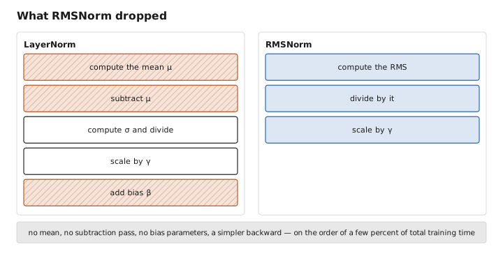
Figure 1. What RMSNorm dropped.
Where to put it: the change that mattered most
The original transformer placed normalization after each sub-block, applying it to the sum of the input and the block’s contribution. The stream would be normalized, passed through attention, added back, and the result normalized again on the way to the next block.
This is a worse arrangement than it appears, and the reason is visible in the residual stream picture. Putting a normalization on the residual path means the path is no longer clean: the gradient travelling back down the tower must pass through a normalization at every level, and the express route that made depth trainable is fitted with a gate at every floor. Models built this way needed a long learning-rate warm-up to train at all, were fragile at depth, and could diverge outright if the warm-up was shortened.
Moving the normalization inside the branch — normalizing the block’s input, leaving the residual addition untouched — fixes it. Now the path from the top of the tower to the bottom is pure addition, exactly as intended, and the normalization only ever guards what feeds into a block rather than what flows between them. Written out, the difference is one set of parentheses:
$$\text{post-norm:}\quad x_{\text{out}} = \text{Norm}\big(x + f(x)\big) \qquad\qquad \text{pre-norm:}\quad x_{\text{out}} = x + f\big(\text{Norm}(x)\big)$$Pre-norm models train stably at depths where post-norm models will not train at all, tolerate much shorter warm-ups, and are far less sensitive to the learning rate. Effectively every large model now uses it.
There is one honest cost, and it follows from the same property that makes it work. Because nothing on the residual path rescales, the stream’s magnitude grows steadily with depth — and since each block reads a normalized copy, a block’s relative contribution shrinks as the stream it is being added to gets larger. Very deep pre-norm models can therefore end up with upper layers whose contributions are, proportionally, barely felt. The usual remedy is a single final normalization at the top of the tower before the unembedding, plus initialization schemes that scale each block’s output down according to depth so that the accumulated total stays sane. Some recent designs go further and normalize on both sides of each block, recovering a little of the post-norm discipline without putting anything back on the residual path.
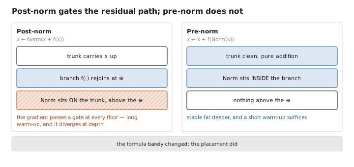
Figure 2. Post-norm gates the residual path; pre-norm does not.
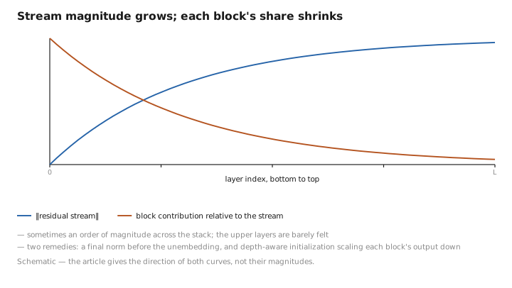
Figure 3. Stream magnitude grows; each block’s share shrinks.
Normalizing inside attention
One further use has become standard and is worth mentioning because it addresses a specific failure rather than a general one.
The scores inside attention are dot products of queries and keys, and nothing constrains their magnitude. Over a long training run, some heads develop very large query or key vectors, the scores grow with them, and the softmax saturates — one weight goes to essentially one, the rest to essentially zero, and the gradient through that head vanishes. The head stops learning, and in the worst case the loss spikes and the run is damaged.
The fix is to normalize the queries and keys before the dot product, capping how large a score can get regardless of what the projections do. This is QK normalization, it costs almost nothing, and it has become common in large models specifically because it removes one of the more frequent causes of a training run falling over at scale. It is a good illustration of what these operations are for: not improving the model’s representations, but keeping the numbers in a range where the rest of the machinery behaves.
What to carry forward
Normalization computes nothing and knows nothing; it exists so that everything else can rely on its input being in a predictable range. Without it, magnitudes drift as the residual stream accumulates, every block finds itself reading a signal unlike the one it adapted to, the distribution moves during training as the layers below change, and the gradient inherits all of it. Layer normalization standardizes across the features of a single token — mean zero, unit variance — then applies a learned per-dimension gain and bias so the model can deliberately depart from the standard if it wants to; computing statistics per token rather than per batch is what makes it usable for variable-length sequences and single-token generation. RMSNorm discards the centring and the bias, dividing only by the root mean square, and matches the full version at lower cost, which is why nearly every recent model uses it. The most consequential decision, though, is placement: normalizing the sum after each block puts a gate on the residual path and produces models that need long warm-ups and break at depth, whereas normalizing the input to each block leaves the path pure addition and trains stably far deeper — at the cost of a stream whose magnitude grows with depth, so that later blocks contribute proportionally less, usually managed with a final normalization at the top and depth-aware initialization. And normalizing queries and keys before the attention dot product caps score magnitudes and prevents the softmax saturation that is one of the more common ways a large training run falls over.
The figures in this article follow the shared figure key , which explains what every shape, line style and colour means.
