A frontier model does not fit on one machine, and the arithmetic makes the point without ceremony: the article on AdamW ’s sixteen bytes per parameter puts a four-hundred-billion-parameter model at six and a half terabytes of training state, against perhaps eighty gigabytes on a single accelerator. Something has to be divided. What makes this more than a logistics problem is that there are five fundamentally different things you can divide — the data, the width of each matrix, the depth of the tower, the sequence itself, and, where the model has them, the experts — and each division has a completely different communication bill attached. Getting the combination right is worth a factor of several in training time, and getting it wrong produces a cluster of expensive machines mostly waiting for each other. This piece is about the five axes and how they are stacked.
The constraint that governs everything
Before the five, the fact that determines all of them. Inside a single machine, accelerators are linked by a dedicated high-speed fabric offering several hundred gigabytes per second and very low latency. Between machines, the link is a network — fast by ordinary standards, and roughly an order of magnitude slower than the fabric inside a box, with far worse latency.
Every parallelism strategy is therefore evaluated not by how much communication it requires in the abstract, but by how much it requires per unit of computation, and whether that communication can be confined inside a single machine. A strategy that talks constantly is fine within a box and ruinous across boxes. This one fact explains nearly every layout choice that follows.
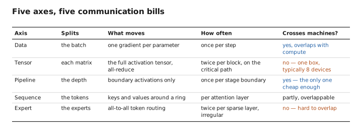
Figure 1. Five axes, five communication bills.
Data parallelism: split the batch
The simplest division. Give every device a complete copy of the model and a different slice of the batch. Each computes gradients on its own slice; the gradients are then averaged across all devices, and everyone applies the identical update.
Communication happens once per step and involves exchanging one gradient per parameter. That is a large volume but a fixed one — it does not grow with batch size — so it amortizes well when each device is doing substantial work, and it overlaps neatly with computation, since the gradients for the last layers are ready while the earlier layers are still being computed. It is the cheapest strategy per unit of throughput and always the first one reached for.
Its limitation is that it does nothing about memory. Every device holds the entire model, so it only helps once the model already fits, and for a large model it does not.
The refinement that changes this is sharding the training state. Notice that a device does not need the optimizer’s running averages for every parameter — it only needs them at the moment it applies the update, and the update for any given parameter could be performed by whichever device happens to own it. So the optimizer state can be split across the data-parallel group, each device owning a slice. Extend the same logic and the gradients can be split too, and then the weights themselves, with each device holding only its shard and gathering the others temporarily when a layer is about to be used. Memory per device falls by roughly the number of devices in the group; the price is more communication, since weights must be gathered before each layer’s forward and backward pass rather than held permanently. This progression — state, then gradients, then weights — is the well-known staged scheme, and its final stage is really a hybrid of data and model parallelism wearing data parallelism’s interface.
Tensor parallelism: split each matrix
Rather than replicating a layer, cut its matrices into pieces and give each device a piece, so that one layer’s computation is performed jointly.
The way the cuts are chosen is elegant, and worth seeing because it minimizes the talking. Take the feed-forward layer , which expands and then contracts. Split the expanding matrix by columns, so each device produces a distinct slice of the hidden activations — no communication is needed, since each device has everything it requires to compute its slice. Apply the nonlinearity elementwise, which is also local. Now split the contracting matrix by rows, matching the way the hidden state was divided. Each device computes a partial result covering the full output width, and the true output is their sum. One addition across devices, and the layer is done.
So a pair of matrices costs exactly one communication rather than two, because the two splits were chosen to compose. Attention is even more natural: distribute whole heads to different devices, since heads are independent by construction, and communicate once when concatenating their outputs.
The bill is one all-reduce per sub-block, which is twice per transformer block, on the full activation tensor. That is a great deal of communication, and it sits on the critical path — nothing can proceed until it completes. Tensor parallelism is therefore used within a machine, across the devices sharing the fast internal fabric, and almost never across machines. In practice this caps the group at the number of accelerators in one box, typically eight.
Pipeline parallelism: split the depth
Give device one the first ten layers, device two the next ten, and so on. Activations flow forward from one device to the next and gradients flow back.
Communication is minimal: only the activations at the boundaries between stages, which is a small tensor compared to anything the other strategies move. This is what makes it the strategy for crossing machine boundaries — it is the only one whose bill is small enough to tolerate a slow link.
Its problem is idleness. If a batch is fed through as a single unit, device two cannot start until device one has finished, and device one has nothing to do while devices two through eight work their way through. The fraction of time wasted is substantial and grows with the number of stages.
The fix is to split the batch into micro-batches and feed them through in sequence, so that once the pipeline is full, every stage is working on a different micro-batch simultaneously. Only the beginning and end of each step have idle stages — the bubble — and its relative size falls as the number of micro-batches rises. With enough micro-batches the waste becomes a few percent. The schedules that interleave forward and backward passes to shrink the bubble further, and to reduce how many activations must be held in flight, are their own small literature.
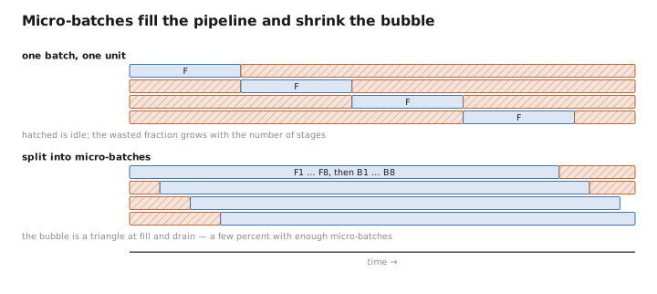
Figure 2. Micro-batches fill the pipeline and shrink the bubble.
Sequence and expert parallelism
Two more axes, each addressing something the first three do not.
Sequence parallelism splits along the token dimension: each device holds a segment of the sequence. This is the answer to long contexts, where the activations for a single example exceed one device’s memory no matter how the model is divided. The difficulty is that attention is precisely the operation that needs every position to see every other, so segments must exchange their keys and values. The standard approach passes them around a ring of devices, so that each segment sees every other’s keys in turn while overlapping the transfer with computation. Operations that are per-token — normalization, feed-forward layers — need no communication at all, which makes this cheaper than it first sounds.
Expert parallelism applies to mixture-of-experts models and places different experts on different devices. Tokens must then travel to wherever their assigned expert lives and their results travel back, which is the all-to-all communication described in that article — twice per sparse layer, with an irregular pattern that depends on the router’s decisions and is therefore hard to overlap. It is also the reason load balancing has a throughput consequence rather than merely a quality one: everyone waits for the device holding the most-requested expert.
A pinch of math: stacking the axes
The strategies are not alternatives; they multiply. If $d$, $t$, and $p$ are the data, tensor, and pipeline degrees, the total device count is
$$N = d \times t \times p$$and the global batch is assembled as micro-batch size times gradient accumulation steps times $d$. Choosing $(d, t, p)$ for a given cluster is the practical exercise, and the reasoning follows directly from the communication costs.
Set $t$ to the number of accelerators inside one machine, and no larger, because tensor parallelism’s per-block all-reduce cannot cross a slow link without dominating. Set $p$ to whatever is needed to make the model’s parameters fit in $t \times p$ devices’ memory, and no larger, because every additional stage enlarges the bubble. Give all remaining devices to $d$, since data parallelism has the best ratio of communication to computation and scales furthest. Then, if activations still do not fit, add sequence parallelism; if the model is sparse, expert parallelism takes the place of some of the tensor degree.
A worked instance makes it concrete. On a thousand accelerators in machines of eight: $t = 8$ confined within each machine, $p = 16$ spanning sixteen machines with the small boundary transfers crossing the network, leaving $d \approx 8$ replicas of that whole arrangement, each processing a different slice of the batch. Communication is heaviest exactly where the fabric is fastest, and lightest where it is slowest, which is the entire design goal.
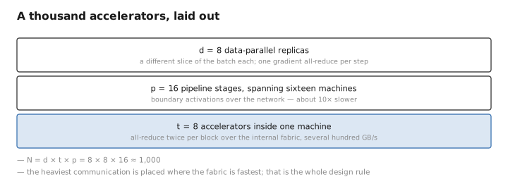
Figure 3. A thousand accelerators, laid out.
What to carry forward
A frontier model’s training state is measured in terabytes and a single accelerator holds tens of gigabytes, so the work must be divided — and the choice of division is governed by one fact, that the fabric inside a machine is roughly an order of magnitude faster than the network between machines. Data parallelism replicates the model and splits the batch, communicating one gradient per parameter once per step, which amortizes well and overlaps with computation but does nothing for memory until the training state is sharded across the group in the staged fashion that splits first the optimizer state, then the gradients, then the weights. Tensor parallelism splits the matrices themselves, choosing column-wise and row-wise cuts that compose so a pair of matrices costs a single all-reduce — but that reduce sits on the critical path twice per block, so it is confined within a machine. Pipeline parallelism splits the depth and communicates only boundary activations, which is small enough to cross machines; its cost is the idle bubble, shrunk by dividing the batch into micro-batches that keep every stage busy. Sequence parallelism splits the tokens, which is how long contexts fit, and requires passing keys and values around a ring so that attention can still see everything. Expert parallelism places experts on different devices and pays the all-to-all that makes load balancing a throughput concern. The five multiply rather than compete, and the standard reasoning is to set tensor degree to a machine’s device count, pipeline degree to the minimum that makes the model fit, and give everything left to data parallelism — placing the heaviest communication precisely where the interconnect is fastest.
The figures in this article follow the shared figure key , which explains what every shape, line style and colour means.
