Two of the better-known methods in post-training define themselves against this one: DPO exists to avoid it, and RLVR is it with the reward model replaced by a checker. The thing itself is worth describing directly. Proximal policy optimization arrived from robotics, where the problem was teaching a simulated body to walk without the training process destroying itself, and it turned out to transfer to language with remarkably little modification. The core difficulty it solves is the same in both settings and is worth stating before any of the machinery: in reinforcement learning, unlike in supervised learning, the model generates its own training data, so a bad update does not merely produce one bad step — it changes what the model will see next, and a policy that has degraded will collect worse experience, from which it will degrade further. Supervised learning is forgiving because the dataset does not move. This piece is about how to take the largest step you safely can when it does.
Why the setup is harder than it looks
Line up what makes this different from ordinary training.
There is no correct answer to imitate. Nobody wrote down the response the model should have produced; there is only a number saying how good the one it produced was. The gradient therefore cannot say “you should have said this” — only “what you said was worth 0.7, and here is how to make things like it more or less likely.”
The reward arrives at the end. A response of five hundred tokens receives one number, and every one of those tokens has to be assigned some share of the credit. This is the credit assignment problem, and it is the reason a naive approach barely works.
The data is generated by the policy being trained. Every update changes the distribution of the next batch. This is what makes the process capable of collapsing, and the collapse can be sudden.
And the reward is a proxy — a learned model of human preference, which as discussed under DPO can be satisfied without the underlying preference being satisfied. Optimizing it hard is not desirable even when it is possible.
The building blocks
The classical answer assembles four pieces, and the ordering below is roughly the order in which each becomes necessary.
Policy gradient. The foundational idea is that you can improve an expected reward by increasing the log-probability of actions in proportion to how much reward followed them. Take samples, weight each token’s log-probability by the reward the sequence earned, ascend. This is correct in expectation and hopeless in practice, because the variance is enormous: two nearly identical responses can receive rewards of 0.9 and 0.2, and the update is dominated by noise.
A baseline. Most of that variance is not about the action taken but about the situation. Some prompts are easy and everything scores well; some are hard and nothing does. Subtracting a prediction of what this situation was expected to yield removes that component without changing the average update. What remains is the advantage: how much better this response was than expected, rather than how good it was.
That prediction has to come from somewhere, and in classical PPO it comes from a critic — a second network, typically initialized from the same model and comparable in size, trained alongside the policy to predict expected return from any partial sequence. This is the piece that doubles the memory of training, the piece DPO removes by deriving its objective differently, and the piece GRPO removes by using the mean reward of a group of samples to the same prompt as the baseline instead.
Advantage estimation over a trajectory. With a critic in hand, the advantage at each token can be estimated in ways that trade bias against variance — from a purely local estimate, which is low-variance but relies entirely on the critic being accurate, to using the full observed return, which is unbiased but noisy. Generalized advantage estimation interpolates between them with a single parameter, and in language-model settings it is usually set near the low-bias end, since the reward genuinely arrives only at the end and there is little intermediate signal for the critic to be right about.
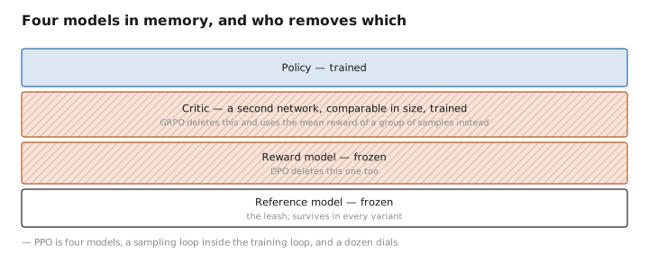
Figure 1. Four models in memory, and who removes which.
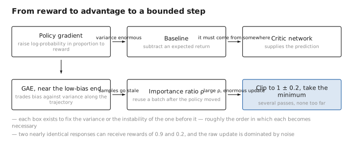
Figure 2. From reward to advantage to a bounded step.
A pinch of math: the clipped objective
The remaining problem is the step size, and this is where PPO earns its name.
Having collected a batch of responses, you would like to extract as much learning from them as possible — several passes of gradient updates rather than one, since generating them was expensive. But those responses were sampled from the policy as it was before any updates. After a few passes the policy has moved, and the samples no longer represent what it would do. Continuing to update on them is drawing conclusions from stale evidence, and it is the classic way for a policy-gradient method to destroy itself.
The correction is importance weighting: scale each token’s contribution by how much more likely the current policy makes it than the sampling policy did.
$$\rho_t = \frac{\pi_\theta(a_t \mid s_t)}{\pi_{\theta_{\text{old}}}(a_t \mid s_t)}$$This is unbiased and it is also the source of the instability, because when $\rho$ becomes large the update becomes enormous — precisely for the tokens the policy has already moved furthest on, which are the ones the evidence supports least.
PPO’s contribution is a blunt and effective fix. Clip the ratio to a narrow band around one, and take the more pessimistic of the clipped and unclipped objectives:
$$\mathcal{L} = \mathbb{E}\Big[\, \min\big(\rho_t \hat{A}_t,\ \ \text{clip}(\rho_t, 1-\epsilon, 1+\epsilon)\, \hat{A}_t \big) \Big]$$with $\epsilon$ usually around $0.2$. Follow it through in both cases and the behaviour is exactly what you want. Where the advantage is positive and the policy has already raised that token’s probability past $1+\epsilon$, the clipped term is smaller, the minimum selects it, and the gradient is zero — no further reward for pushing something you have already pushed enough. Where the advantage is negative and the probability has already fallen below $1-\epsilon$, the same thing happens in reverse. But if the ratio moves the wrong way — the policy made a good token less likely — the unclipped term is selected and the full correction applies, because there is no reason to limit a step that is fixing a mistake.
The result is a method that permits multiple passes over each expensive batch of samples while structurally refusing to move too far on any one of them. No trust region has to be computed, no constrained optimization solved. It is one clip and one minimum, and its ratio of practical value to conceptual complexity is about as high as anything in the field.
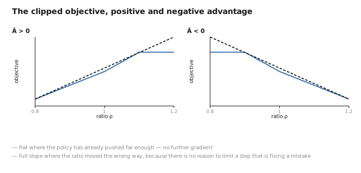
Figure 3. The clipped objective, positive and negative advantage.
The language-model specifics
Applied to text, several additions become standard.
The KL penalty to the reference model is the leash, and as the article on KL divergence explains it is used in the mode-seeking direction deliberately: the policy is forbidden from putting mass where the starting model saw none, while being free to narrow. It is applied per token as a subtraction from the reward rather than as a term in the loss, which lets the advantage machinery handle it. Its coefficient is the single most consequential dial in the setup, and some implementations adapt it during training to hold the observed divergence near a target.
Whitening the advantages within a batch — subtracting the mean and dividing by the standard deviation — is close to universal and matters more than its triviality suggests, since reward models produce scores on an arbitrary scale that drifts as training proceeds.
Value function initialization is a real difficulty. The critic starts knowing nothing, so its early predictions are poor, so early advantages are mostly noise, at exactly the moment the policy is most impressionable. The usual mitigations are to warm up the critic before updating the policy, or to initialize it from the reward model, which at least has a notion of what good looks like.
And reward hacking remains the standing failure mode, arriving in the specific forms that article described: length inflation, formulaic structure, sycophancy. The KL penalty limits it; it does not prevent it.
Where it stands now
PPO is more expensive and more finicky than the alternatives — four models in memory, a sampling loop inside the training loop, and a dozen interacting dials — and for a period it looked as though DPO had made it obsolete. That is not how it turned out.
Two things kept it in use. It is genuinely on-policy, learning from what the current model actually produces rather than from a fixed dataset, which is the property DPO gives up and the one that matters most as training proceeds and the policy drifts from the data. And when the reward is a program rather than a learned model, the objection that motivated much of the retreat from RL simply evaporates — a checker cannot be hacked in the way a reward model can, so the leash can be loosened and the optimization pushed hard. That is exactly the situation of verifiable rewards , and it is why reinforcement learning came back into the centre of post-training just as it seemed to be leaving. What changed is mostly the critic: GRPO’s group-relative baseline removed the most expensive component while keeping the clipped objective intact, so what runs today at scale is recognizably PPO with one piece taken out.
What to carry forward
Reinforcement learning on a language model is harder than supervised training because there is no correct answer to imitate, the reward arrives only at the end of a long response, and the model generates its own training data — so a bad update degrades the experience collected next, and the failure can compound. The machinery builds up in stages: policy gradient raises the log-probability of tokens in proportion to the reward that followed, which is correct and far too noisy; a baseline subtracts what the situation was expected to yield, converting reward into advantage and removing most of the variance; and in classical PPO that baseline comes from a critic network the size of the model, which is the component both DPO and GRPO were built to eliminate. The method’s own contribution is the clipped objective: importance-weight each token by how much more likely the current policy makes it than the policy that sampled it, then clip that ratio to a narrow band and take the pessimistic branch, so that a token already pushed far enough yields no further gradient while a correction in the wrong direction is still applied in full. That single device allows several update passes over each expensive batch without any one of them moving too far. In language settings it is joined by a per-token KL penalty to the reference model — the leash, in the mode-seeking direction — advantage whitening, and careful critic initialization. It looked superseded by DPO’s simplicity, and it was not: it is genuinely on-policy, and when the reward is a verifier rather than a learned proxy the case against hard optimization disappears, which is why what runs at scale today is this method with the critic removed.
The figures in this article follow the shared figure key , which explains what every shape, line style and colour means.
