Ask why language models are trained to predict the next word and the answers tend toward the grand: that language is produced sequentially, that prediction is compression and compression is understanding, that anticipating what comes next is what a mind does. None of that is exactly wrong, and none of it is the reason. The objective won a competition against several serious rivals, on grounds that were largely accounting — how much learning can be squeezed out of each token of text, and out of each unit of compute. For a couple of years around 2018 the favourite was something else entirely. Why the sums came out as they did explains a good deal that otherwise looks arbitrary: why encoder models still beat decoders at certain jobs, why a model is never trained in the situation it is deployed in, and why a handful of losing objectives survive in particular corners. This piece is about the constraint that forced the choice, the arithmetic that settled it, and what the field gave up in exchange.
There are no labels, and nobody is going to annotate a trillion tokens
Every supervised method needs a target to compare its output against, since gradient descent only reduces a discrepancy between prediction and answer. The text required to train a competent language model runs to trillions of tokens. Those two facts do not sit together. No conceivable annotation effort produces labels at that scale, and if one did, the labels would encode whatever narrow task the annotators were briefed on rather than the general competence wanted.
So the objective has to manufacture its own supervision out of the raw material. This is self-supervision, and the trick in every version is the same: hide part of the input, and require the model to reconstruct it from what remains. The text becomes both question and answer. No human is involved, the signal is limited only by the supply of documents, and assembling a corpus becomes a matter of filtering rather than labelling.
That leaves a design space with two axes, which is where the real argument lives: what to hide, and how much. Every answer defines a different task, and every task is a proxy — a word doing serious work in that sentence. You are not training the thing you want. You are training on a task whose solution you hope requires it, and that gap is never closed by argument, only by results.
Density is what settled the argument
The rival formulation, for a while the more respectable one, was masked language modelling: replace roughly fifteen percent of the tokens with a placeholder, let the model read the mutilated sequence in both directions, and ask it to recover what is missing. It produced the encoder models that dominated benchmark tables for several years. It lost anyway, for two reasons worth separating.
Every position is a training example. A causal model reads a sequence of a thousand tokens and is scored at all thousand positions — the second token given the first, the third given the first two, and so on to the end. Each is a real prediction with a real target, each contributes a term to the loss, and all come out of one forward pass, because the causal mask stops any position seeing its own successor while leaving it free to see everything before. Nothing is wasted. The masked objective takes a gradient only at the corrupted positions, fifteen tokens in every hundred; the other eighty-five are read, processed at full cost, and scored not at all. Six or seven times less signal for the same compute.
The obvious repair does not work, which is what makes this decisive rather than incidental. Masking more would raise the density, but the masked positions are predicted from the unmasked ones, and past some fraction there is not enough context left. The task destroys its own premises. Fifteen percent is roughly where the trade bottoms out. Only by sweeping the corruption rate across the whole range, up to and including everything, does the objective turn into something else — the manoeuvre diffusion language models rest on, and it took years to make it pay.
Generation comes free. A model trained to predict the next token is already a generator: sample from its output distribution, append the result, run it again. There is nothing to add. A bidirectional model has no such property, never having been asked to produce a token at a position it could not see, so generating from it needs a procedure bolted on afterwards, and every such procedure is awkward. The decoding machinery everything now depends on exists because the objective handed it over at no cost. That was not the argument in favour at the time. It became the argument that mattered.
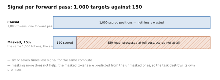
Figure 1. Signal per forward pass: 1,000 targets against 150.
A pinch of math: the chain rule, and one term per position
The reason the causal objective is so tidy is that it is not an approximation of anything. Take a sequence $x_1 \ldots x_n$ and write its joint probability by repeatedly conditioning:
$$p(x) = \prod_{t=1}^{n} p(x_t \mid x_{The task looks small, and the field cannot agree how small it is
Predicting one word from the words before it sounds like the least ambitious demand one could make of a large network. The defence, sound as far as it goes, is that the only way to do it well across a very great many tokens is to represent whatever determines those tokens. Closing a bracket requires tracking that one was opened. Choosing the verb form requires the subject. Continuing a proof, a stack trace or a legal clause requires enough of the content to know what follows from it. The objective places a bounty on any regularity at all that reduces surprise, and is entirely indifferent to what kind.
The deflationary reading is also true and belongs in the same breath. An enormous share of what the objective rewards is surface statistics — which word usually follows which, how a template completes, what a document of this shape contains next. Those tokens are numerous and cheap, and because the loss is an average over positions, they dominate it. A model can improve substantially on the metric while getting no better at anything a person would notice, which is why evaluation is a separate discipline.
The interesting disagreement sits on the boundary between those accounts, and it has not moved much. One position holds that surface statistics are scaffolding and the residual is where the substance accumulates. The other holds that the residual is smaller than it looks, and that most apparent reasoning is retrieval of a pattern seen in training. The aggregate loss cannot separate them, since it sums over positions without labelling any, and the experiments that might are contested.
What the choice costs, and where the middle paths survive
The bill for choosing causal was presented immediately and paid deliberately.
Every representation is built blind to what follows. At position forty of a sentence, a causal model has seen thirty-nine tokens; a bidirectional encoder at the same position has seen the whole sentence. That is strictly more information, and for any task consuming a representation instead of continuing a text — classification, sentence similarity, the vector lookups behind retrieval — the encoder held a real advantage for years, and for some of these jobs the specialists have never been displaced. The workarounds — take the final position’s state and hope it summarizes, or reopen the mask later — are unlovely. The field traded representational quality for scale and generation, knowingly.
Training never visits the situation the model is deployed in. Under teacher forcing, every prediction during training is conditioned on the true, human-written prefix, because the target sequence is right there and using it is what makes the parallel computation possible. At generation time the prefix is the model’s own output. Those are different distributions, and the gap is called exposure bias: a model that has drifted somewhere slightly odd is conditioning on text unlike anything it was trained on, its next prediction is worse, and errors compound in a regime training never entered. Much of what later training stages accomplish is dragging the model toward the conditions of its own use. That this is still necessary indicts the objective.
The rival objectives survive where the cost bites. Span corruption masks contiguous runs and asks the model to emit them in order: denser than token masking, still bidirectional over the input, generative in a limited way. Prefix objectives let the model read one portion with full bidirectional access and predict the rest causally. Fill-in-the-middle rearranges a document so the ending precedes the gap, teaching an ordinary causal model to condition on both sides — standard in code completion, where the text below the cursor is right there and ignoring it would be absurd. None displaced the plain causal loss, and all persist where its demands are not met. The monopoly is a practical outcome, arrived at by measurement, not a proof that the alternatives were wrong.
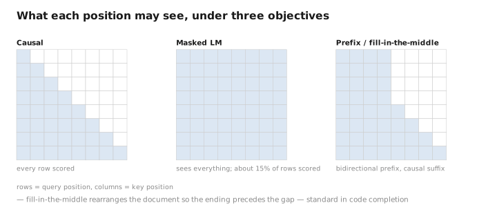
Figure 2. What each position may see, under three objectives.
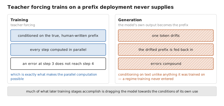
Figure 3. Teacher forcing trains on a prefix deployment never supplies.
What to carry forward
The objective was chosen under a constraint easy to forget once the models exist: no labels exist at the scale required, and nobody was ever going to annotate a trillion tokens, so the task had to be built out of the text itself by hiding part of the input and demanding its reconstruction. What separates the candidates is signal per token read, and predicting the next token extracts the maximum available — a thousand-token sequence yields a thousand scored predictions from one forward pass, because a causal mask lets every position see its predecessors and not its successors. Masking fifteen percent of positions instead yields a gradient at fifteen tokens in a hundred while paying full price to process the rest, and cannot simply mask more, since the masked tokens are predicted from the unmasked ones. Generation then arrives free, a next-token predictor sampled repeatedly being already a generator, where a bidirectional model needs one invented for it. Underneath sits the chain rule of probability, an exact identity rather than a modelling assumption, which is why the causal loss corresponds to a real sequence probability and the masked one does not. What was paid for that: a representation built with no knowledge of what follows, strictly less than a bidirectional encoder has, which is why encoders long remained better at classification and retrieval and in places still are; and a training regime that always conditions on human-written text while deployment conditions on the model’s own, so errors compound in a distribution training never visited. Span corruption, prefix objectives and fill-in-the-middle survive exactly where those costs bite hardest. The monopoly is an empirical result about signal per unit of compute, not a discovery about language, and nothing has established that the argument was settled correctly for any purpose other than scale.
The figures in this article follow the shared figure key , which explains what every shape, line style and colour means.
