Anyone who learned this subject from the textbooks of the twenty-tens learned that the central hazard of fitting a flexible model to data was overfitting, and learned an apparatus for holding it off: a penalty on the size of the weights, noise injected into the activations, a held-out split watched for the moment its curve turns up, augmentation to manufacture examples the collection lacked. That training was sound and the techniques worked. Then you read a technical account of a large language model and find almost none of it. No noise injection. No stopping criterion based on held-out loss, because nothing turns upward to stop at. A weight decay coefficient, retained, listed among the settings with no explanation beyond its value. The tempting conclusion — that the received wisdom was wrong, or that scale makes carelessness affordable — is not what happened. This piece is about which precondition stopped holding, what the surviving weight decay is actually doing, and what took over the job the old defences performed.
The received picture was correct about a setting that no longer obtains
Begin with the classical account, because it describes something real. Take a collection of some tens of thousands of examples and a model with far more capacity than the collection can pin down, and train it as long as you like. The training loss falls and keeps falling, because there is always some further contortion that fits the examples in front of it a little better. The held-out loss falls too, for a while, then bottoms out and rises. Past the turning point the model is learning the noise in the sample rather than the structure behind it.
The apparatus exists to manage that curve, and each piece attacks it differently. A penalty on the norm of the weights makes the contortions expensive, so the fit has to earn its complexity. Injected noise stops any unit from relying on the precise behaviour of its neighbours, since the neighbour may not be there. Augmentation enlarges the sample with transformations that ought not to change the answer. And a held-out split supplies what all of it needs: a signal for where the turning point is, which the training loss will never give.
None of this was mistaken and none of it has been refuted. What is easy to miss is that the argument was conditional. It assumed a model with more capacity than the data could constrain, and enough passes over that data for the model to start fitting its idiosyncrasies. Both conditions were so dependable that nobody stated them. One has stopped being true.
One pass over a corpus larger than the model changes the binding constraint
A large language model is trained for roughly a single pass over a corpus containing far more text than it has parameters to store. Most training examples are seen once and never again. There is no second epoch in which the model can memorize what it saw in the first, because for the bulk of the data there is no second epoch at all.
So the classical curve is not what practitioners observe. The held-out loss does not turn upward. It goes down, more and more slowly, in the regular way that scaling laws describe, until the compute budget runs out and the run stops. The binding constraint has moved. In the old setting the scarce resource was data and the model was large relative to it; now the data is effectively inexhaustible and the scarce resource is arithmetic. Scaling laws are the statement of that second regime, which is why they say nothing about when to stop and everything about how to spend.
This is where dropout went. It was standard in the models of the twenty-tens and is largely absent from large pretraining runs, and the reason is mechanical rather than fashionable. Dropout injects noise that prevents units from co-adapting on data they will meet again, and it charges for the service: the network trains as a blurred ensemble of subnetworks, giving up effective capacity, and converges more slowly because each step is taken on a degraded model. In a data-limited setting that is an excellent trade. In a single-pass, compute-limited setting it pays a real price in the scarce resource to suppress a failure that is not occurring. Dropout has not left the field, though, only pretraining. It survives wherever the old preconditions hold — fine-tuning on a few thousand examples for many epochs, with a model vastly larger than the task needs, which is the classical picture exactly.
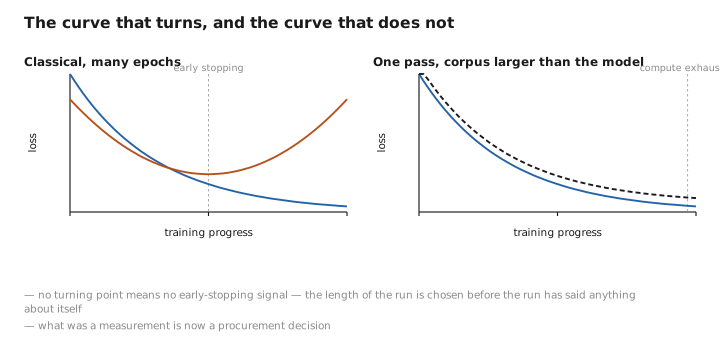
Figure 1. The curve that turns, and the curve that does not.
Weight decay survived, and it is not doing what its name suggests
Weight decay did not follow dropout out of the door, which is odd if its purpose was capacity control, since the argument for dropping dropout applies word for word. Something else is going on.
Two clues. The first is that in the optimizer these models are trained with, the decay is not a term in the loss; it is a separate shrinkage applied to every weight after the gradient step, kept deliberately outside the adaptive rescaling. Any intuition inherited from treating it as a prior is already strained by that surgery. The second is that removing it does not produce the signature of failed regularization. Runs without decay do not fit their training data suspiciously well; they optimize worse.
The reading that fits the evidence is that decay controls the scale of the weights, and the scale of the weights controls the effective size of a step. A learning rate is a fixed absolute quantity, so as a weight matrix grows in norm the same step becomes an ever-smaller relative change to what the layer computes, and the model gradually stops moving while appearing to train normally. Decay puts a ceiling on that growth and keeps the relative step size roughly stationary over a long run. On this account it is not preventing memorization; it is maintaining the conditions the optimizer needs to keep making progress, which places it nearer to a normalization trick than to a penalty. Accounts of the mechanism differ and the argument is unsettled. The empirical fact is not: the coefficient earns its place in every configuration file, and the explanation printed beside it is not the reason.
A pinch of math: two objectives, and a dial that moves when you move another
Put the two readings side by side; the difference is one line of algebra.
The classical form adds a penalty to the objective:
$$L(\theta) + \frac{\lambda}{2}\lVert\theta\rVert^2$$and the reading follows from the shape. Any setting of the parameters must justify its norm by the loss it buys, so large-norm solutions are excluded unless they fit substantially better — the hypothesis space is shrunk, and $\lambda$ says by how much.
The decoupled form does not touch the objective. It shrinks the weights directly, alongside whatever step the optimizer computed from the gradient estimate $\hat{g}$:
$$\theta \leftarrow \theta - \eta\,\hat{g} - \eta\lambda\theta$$Now look at the last term. The shrinkage is multiplied by the learning rate $\eta$, so each step retains a fraction $(1 - \eta\lambda)$ of every weight — a fraction set by a quantity belonging to the gradient half of the update. Decay the learning rate, as every schedule does, and you have weakened the regularization by the same factor, at exactly the point where the classical story says restraint matters most. The penalized objective predicts nothing of the kind: there, $\lambda$ describes the problem and $\eta$ describes only how fast we solve it. Here the two are welded, and the welding follows from the update rule rather than from any argument about generalization. Decoupling bought independence from the per-parameter gradient scale and left this entanglement standing. So the effective strength of the decay is a product of two dials, not the number in the configuration.
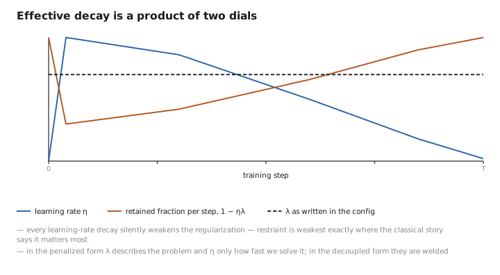
Figure 2. Effective decay is a product of two dials.
What took over the job, and what it quietly fails to do
If the old defences are gone and the loss still behaves, something is doing the work. Three things are, and none is a term in the objective.
Deduplicating the corpus does the most. The web repeats itself relentlessly, and a document appearing forty times in the raw crawl is forty opportunities to spend capacity on a specific string rather than on the language around it. Removing them removes the only part of a single-pass regime that behaves like multiple epochs. Notice what kind of intervention that is: it fixes the data rather than constraining the model, and it belongs to the mixture pipeline, not the optimizer.
The noise in the gradients regularizes for free. Each step is taken on an estimate assembled from a sample, and the resulting jitter keeps the parameters from settling into narrow crevices of the landscape. Nobody adds it and nobody pays for it. But it shrinks as the batch grows, so a very large batch removes a stabilizer along with the variance — one of several reasons the largest batches disappoint at equal data.
And the corpus itself is the real defence. A model cannot memorize its way to a low loss on a trillion tokens it will see once, because the capacity is not there and the second look is not coming. That is the least elegant answer available and the load-bearing one.
None of that prevents memorization. The absence of the classical curve is easily misread as evidence that nothing is being stored. Verbatim retention of rare sequences happens, it is measurable, and it is a different phenomenon from the aggregate loss, which is an average over billions of tokens and insensitive to a few thousand of them. The reassuring curve and the memorization problem coexist comfortably.
And nothing tells you when to stop. Early stopping was a decision made on evidence: watch the held-out curve, halt at the minimum. Where the curve never turns, that evidence does not exist. The endpoint is fixed instead by the budget and written into a schedule that must reach zero on time, so the length of a run is chosen before the run has said anything about itself. What was a measurement is now a procurement decision.
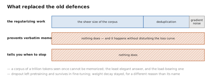
Figure 3. What replaced the old defences.
What to carry forward
The classical account of overfitting was correct about a setting defined by two conditions so dependable that nobody wrote them down: a model with more capacity than the data could constrain, and enough passes over that data for the model to begin fitting the sample rather than the structure. Large-scale pretraining satisfies neither. Roughly one pass over a corpus far larger than the model means most examples are seen once and there is no second epoch in which to memorize the first, so the held-out loss does not turn upward — it falls until the arithmetic runs out, which is what makes the regime compute-limited rather than data-limited and what the scaling laws describe. Dropout left because it charges effective capacity and slower convergence to suppress co-adaptation on repeated data, and there is no repeated data; it remains sensible in fine-tuning on small collections, where the old conditions hold exactly. Weight decay stayed, and its name has outlived its mechanism: applied as direct shrinkage outside the loss, its benefit looks less like capacity control than like keeping the norm of the weights bounded so that a fixed learning rate remains a meaningful relative change — an explanation still contested, over an effect that is not. Its strength is multiplied by the learning rate, so every decay of the schedule quietly weakens it. What performs the old function now is deduplication, gradient noise that thins as batches grow, and the sheer size of the corpus, the least elegant of the three and the one carrying the weight. None of them guarantees anything against verbatim retention, which happens without disturbing the loss curve, or supplies a signal for when to stop, which is now set by a budget fixed before the evidence exists.
The figures in this article follow the shared figure key , which explains what every shape, line style and colour means.
