The article on embeddings concerned the table at the bottom of a language model, which turns each token into a vector so the tower has something to work with. The object here is a different one with an unfortunately identical name: a model whose entire output is a single vector representing a whole passage, built so that passages about the same thing land near each other and can be found by searching. The two share a word and a geometric intuition and almost nothing else. The distinction is worth insisting on, because a great deal of confusion in practice comes from expecting one to do the other’s job — and in particular from the reasonable-seeming and wrong idea that a good language model must contain a good search index. This piece is about why it does not, what the training objective actually asks for, and what the resulting vectors cannot be made to do.
Why a language model is not one
Suppose you want to find, among a million passages, the one that answers a question. The obvious thought is to use the model you already have: run each passage through it and take some summary of the internal state as its representation.
This works badly, and the reason is instructive. A language model is trained to predict the next token. Its internal state at any position is optimized to be useful for that prediction, which means it is dominated by local, syntactic, immediately-relevant information — what part of speech is coming, which entity is currently in play, whether a clause is closing. It is not optimized to summarize a passage in a way that supports comparison with other passages. Nothing in the training objective ever asked for that.
There is a more specific problem. Averaging a model’s token representations produces vectors that are all rather similar to one another, because they share the dominant directions that every position carries — the anisotropy noted in the article on embeddings , where learned representations occupy a narrow cone rather than spreading out. Similarity scores computed this way are all high and differ in the third decimal place, which is a poor foundation for ranking a million candidates.
A retrieval model is therefore trained separately, for a different objective, and usually initialized from an encoder -style architecture that reads bidirectionally rather than left-to-right — because a passage being summarized is available all at once, and there is no reason to hide its second half from its first. The construction that follows is the same one that, applied across modalities rather than within one, produces the vision encoders of multimodal models .
What the training objective actually is
The requirement is easy to state: a question and its answer should be close; a question and an unrelated passage should be far. The training method that achieves it is contrastive, and its central quantity is not similarity but relative similarity.
Take a batch of question-passage pairs known to belong together. For each question, its own passage is the positive and every other question’s passage in the batch is a negative. Then apply a softmax over the similarities and maximize the probability of the correct one:
$$\mathcal{L} = -\log \frac{e^{\,\text{sim}(q, p^{+})/\tau}}{\sum_{j} e^{\,\text{sim}(q, p_j)/\tau}}$$This is cross-entropy over a set of candidates rather than over a vocabulary, and reading it that way makes the design decisions legible.
The objective is about ranking, not about absolute distance. Nothing requires the correct pair to reach any particular similarity; it only has to beat the alternatives. This is why the scores such a model produces are not calibrated and should not be thresholded as if they were probabilities.
The temperature $\tau$ does what it does everywhere: a small value sharpens the distribution and concentrates the gradient on the hardest negative, a large one spreads it. It matters more here than in most places, and is typically small.
And the negatives are the whole game. Random passages are trivially distinguishable — a question about tax law versus a passage about volcanoes teaches almost nothing after the first few steps. What produces a good model is hard negatives: passages that look relevant and are not. The standard method is to retrieve candidates with a current version of the model, discard the true positives, and train against the highest-ranked remainder, iterating as the model improves. Since negatives are shared across the batch at almost no extra cost, larger batches supply more of them, which is why these models are trained with unusually large batches and with mechanisms for holding many more negatives in memory than the batch itself contains.
The other lever is symmetry. Questions and passages look nothing alike — one is short and interrogative, the other long and declarative — so many systems use two separate encoders, one per side. Others use a single model with a short instruction prefixed to each input telling it which role it is playing, which is simpler to serve and works about as well.
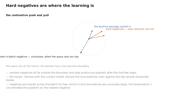
Figure 1. Hard negatives are where the learning is.
Bi-encoders and cross-encoders
There are two ways to score a query against a passage, and the difference between them determines the shape of every retrieval system.
A bi-encoder encodes each independently and compares the resulting vectors. The passage vectors can be computed once, in advance, for the entire corpus. At query time only the question must be encoded, and the search is a nearest-neighbour lookup among precomputed points. This scales to billions of documents.
A cross-encoder takes query and passage together as one input and outputs a relevance score. Attention runs across both, so every word of the question can interact with every word of the passage — which is far more accurate, because relevance often depends on a specific correspondence that no independent summary of either side can preserve. It also means nothing can be precomputed: every query-passage pair requires a full forward pass, so scoring a million passages requires a million forward passes.
The resolution is the two-stage arrangement described under RAG . A bi-encoder retrieves a few hundred candidates cheaply from the whole corpus; a cross-encoder reranks those few hundred expensively. Cost scales with the corpus for the cheap stage and with the shortlist for the accurate one. Between the two sits a middle option that keeps a vector per token rather than per passage and computes a fine-grained match at query time — more accurate than a single vector, far cheaper than full cross-attention, and considerably more storage.
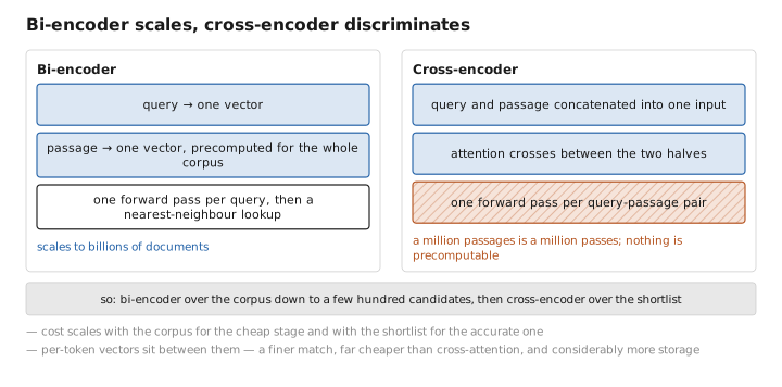
Figure 2. Bi-encoder scales, cross-encoder discriminates.
What the vectors cannot do
Three limitations are worth knowing because they explain most disappointing results.
Exact matching is a weakness, not a strength. A dense vector represents a passage approximately, which is what lets it match paraphrases — and it is exactly wrong for finding a specific product code, an unusual surname, an error string, or a rare technical term. Traditional keyword search handles those perfectly and handles paraphrase not at all. The two are complementary in the strict sense, which is why serious systems run both and merge the rankings, an arrangement usually called hybrid search. Reaching for dense retrieval alone because it is newer is a common and easily avoided mistake.
A single vector is a bottleneck. A long passage covering several topics gets one point in space, which is an average of its contents and therefore near nothing in particular. This is really an argument about chunking: passages should be short enough that one vector honestly represents them.
Relevance is not one thing. The model has learned some particular notion of relatedness from its training pairs, and a query may want a different one — the most recent document, the most authoritative, the one from the right jurisdiction, the one that contradicts rather than matches. None of these are geometric properties of a semantic embedding, and expecting a vector search to honour them leads to protracted confusion. They belong in metadata filters and in ranking logic outside the vector.
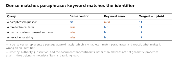
Figure 3. Dense matches paraphrase; keyword matches the identifier.
Practical matters
Two brief points that come up immediately in use.
Searching a billion vectors exactly is too slow, so approximate methods are used — layered proximity graphs are the common choice — which trade a small chance of missing a true nearest neighbour for enormous speed. The recall loss is usually negligible next to the errors the embedding model itself makes.
And storage is real: a billion passages at a thousand dimensions in four bytes is four terabytes. The vectors compress well, since retrieval needs only relative ordering rather than precise values, and the same quantization logic applies. Some models are now trained so that a prefix of the vector is usable on its own, which allows searching cheaply on a truncated version and refining with the full one — the same coarse-then-fine pattern as the two-stage pipeline, applied within a single vector.
What to carry forward
A retrieval embedding is a separate model from the token embedding table it shares a name with: it maps a whole passage to one vector chosen so that related passages land near each other. A language model’s internal states do not serve this purpose, because they are optimized to predict the next token rather than to summarize a passage for comparison, and because they occupy a narrow cone that makes all similarities look alike. The training is contrastive — a softmax over candidates in which a question’s own passage must outrank every other, which makes the objective about relative ranking rather than absolute distance, so the scores are not calibrated and should not be thresholded as probabilities. Its quality is determined largely by the negatives: random passages teach nothing after the first steps, so systems mine hard negatives by retrieving with the current model and training against the top-ranked wrong answers, iterating, and they use very large batches because negatives are shared across a batch for free. Scoring comes in two forms — a bi-encoder that embeds each side independently, allowing the corpus to be precomputed and searched at scale, and a cross-encoder that reads query and passage together for far better accuracy at a cost that scales with the number of pairs — which is why the standard pipeline retrieves broadly with the first and reranks narrowly with the second. The limitations follow from what a dense vector is: it is approximate, so it matches paraphrases well and exact identifiers badly, which is why hybrid search with keyword matching is standard; one vector per passage is a bottleneck that argues for short chunks; and notions of relevance like recency, authority, or contradiction are not geometric and belong outside the vector entirely.
The figures in this article follow the shared figure key , which explains what every shape, line style and colour means.
