There is something peculiar about the fact that this works at all. A neural network is a chaotic object — billions of parameters set by a stochastic process, on data nobody has fully inspected, through an optimization that visits an incomprehensible landscape. Nothing about that description suggests predictability. And yet the loss such a model achieves is a smooth, regular function of three numbers: how large it is, how much it read, and how much arithmetic was spent. Plot loss against any of them on logarithmic axes and you get a straight line, holding over many orders of magnitude. This is what makes it possible to spend a hundred million dollars on a training run with any confidence about the outcome, and it is the closest thing the field has to a physical law. This piece is about the relationship, the correction that reshaped the field’s spending, and the ways the law is more limited than its elegance suggests.
The shape of the relationship
Hold everything else fixed and vary one quantity — parameters $N$, training tokens $D$, or total compute $C$ — and the loss follows a power law with an offset:
$$L(N) = \frac{A}{N^{\alpha}} + L_\infty$$Two parts, and both matter. The power-law term is the reducible loss, and it falls steadily but with diminishing returns: each halving of the loss above the floor costs a multiplicative increase in scale, not an additive one. The offset $L_\infty$ is the irreducible loss — the entropy of language itself, as the article on cross-entropy described, which no model can cross because text is genuinely not deterministic.
The remarkable properties are the empirical ones. The exponents are small, which means progress is slow but extraordinarily reliable — though the precise values depend entirely on how the curve was fitted, and quoting them across papers is a trap. Fits that absorb the irreducible floor into the power law report exponents around $0.05$ to $0.1$; fits that subtract an explicit floor first, and so describe only the reducible part, report around $0.3$. The two are not comparable, and most published disagreement about “the” exponent is this distinction rather than a disagreement about the data. The relationship holds across many orders of magnitude with very little scatter. And it is largely insensitive to architectural detail — depth against width, the precise attention variant, most of the choices practitioners argue about move the curve by a small constant factor rather than changing its slope. Scale dominates, and it dominates by so much that the correct first response to “will this architectural change help?” is usually “less than making the model bigger.”
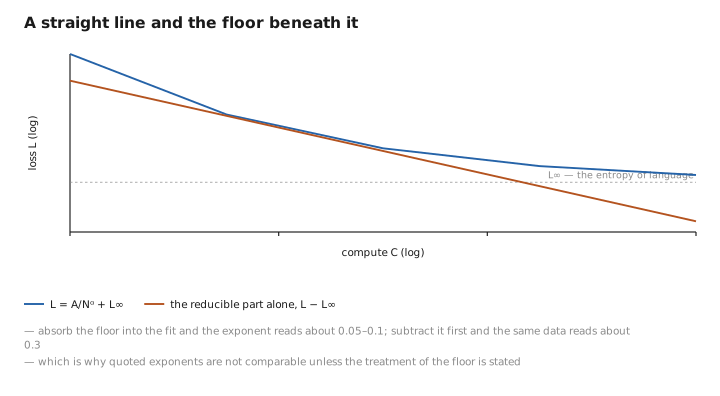
Figure 1. A straight line and the floor beneath it.
The correction that moved a billion dollars
The first influential formulation, from 2020, examined how a fixed compute budget should be divided between model size and training data, and concluded that model size deserved most of it. Roughly, if compute increases tenfold, make the model about five times larger and train it only about twice as long. The industry followed, and the era of enormous, briefly-trained models followed with it: models of a hundred and seventy-five billion parameters trained on a few hundred billion tokens, barely more than one token per parameter.
Two years later a careful re-examination found this was wrong, and the reasons are a lesson in themselves. The correcting paper pointed to a learning-rate schedule that did not decay properly for shorter runs, making those runs look worse than they were and so making training longer look less valuable than it was. Later work has revised that diagnosis: the largest single factor appears to be that the original counted non-embedding rather than total parameters, and fitted at small scale where that distinction matters most, with warm-up duration and scale-dependent optimizer settings contributing the rest. The specific culprit is still argued over. What is not argued over is the shape of the failure — a set of methodological choices in ancillary settings, none of them the object of study, misdirected the field’s largest expenditure for two years.
The corrected result is that parameters and tokens should scale in equal proportion. Double the compute and you should make the model about $1.4$ times larger and train it on about $1.4$ times more data — not five times larger and twice as long. The compute-optimal ratio works out to roughly twenty tokens per parameter, and the demonstration was direct: a seventy-billion-parameter model trained on 1.4 trillion tokens outperformed a model four times its size across the board, using the same compute.
The reason the arithmetic comes out this way is straightforward once seen. Training compute is approximately
$$C \approx 6ND$$— six floating-point operations per parameter per token, two for the multiply-add in the forward pass and roughly twice that again for the backward pass. So $N$ and $D$ enter the budget symmetrically. If the loss also responds to them with similar exponents, which it approximately does, then symmetry in the cost and symmetry in the benefit means they should be scaled together. The earlier asymmetric recommendation had implied the exponents were quite different, and the flawed schedule was what created that impression.
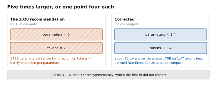
Figure 2. Five times larger, or one point four each.
The twist: training-optimal is not serving-optimal
The correction was quickly followed by a realization that complicates it, and that now governs how most deployed models are built.
Compute-optimal answers the question what is the best model I can train for this budget. Almost nobody actually wants the answer to that question. What they want is the best model they can afford to run, and inference cost is paid per request, forever, by everyone. A smaller model is cheaper on every single query it will ever serve.
So it is rational to deliberately overshoot the token count — to train a smaller model on far more data than the compute-optimal ratio recommends, accepting a worse loss for the training budget in exchange for a permanently cheaper model. The loss curve is quite flat in this region, so the sacrifice is modest and the saving is not. This is why models are now routinely trained at hundreds or even thousands of tokens per parameter, an order of magnitude past twenty. The Chinchilla ratio is the right answer to a question that most people are not asking.
The correct framing is total cost of ownership: training compute plus expected lifetime inference compute. Under that objective the optimal model is smaller and better-read than the compute-optimal one, and how much smaller depends on how many requests you expect to serve — which is a business forecast rather than a scientific quantity.
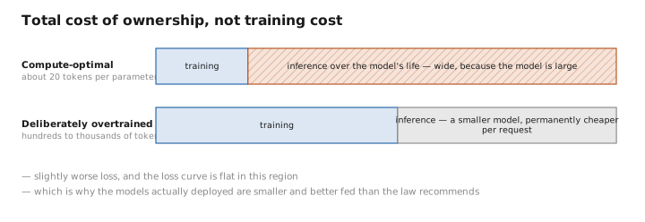
Figure 3. Total cost of ownership, not training cost.
What the law does not tell you
Four honest limitations, because the relationship is often extended past where it has been established.
It predicts loss, not capability. The smooth curve describes cross-entropy on held-out text. What people care about is whether the model can do things, and the mapping from one to the other is not smooth. Performance on specific tasks has repeatedly appeared to jump at particular scales rather than improving gradually — the phenomenon called emergence . There is a good deflationary argument that much of this is an artifact of measurement: a metric like exact-match accuracy is a threshold on an underlying continuous quantity, and a smoothly improving probability of getting every step right will look like a sudden jump when you only score complete successes. Where the sharpness is real and where it is the scoreboard remains genuinely contested, and either way the practical point stands — the loss curve will not tell you at what scale a capability appears.
The exponents are properties of the data. A scaling law is fitted on a particular corpus and describes that corpus. Change the data mixture , the filtering strictness, or the repetition rate and the constants move. Improving the data shifts the entire curve down, which is a more valuable thing to do than moving along it, and is invisible to a law fitted before the change.
Repetition breaks it. The relationship assumes fresh tokens. As discussed under data mixtures, repeated data is nearly as good as new up to about four passes and rapidly less so thereafter, so the token axis stops meaning what it meant once you are recycling.
It says nothing about post-training. Everything here concerns pretraining loss. Reasoning models added a second axis entirely — compute spent at inference time, which trades against model size in a way no pretraining law anticipated — and the scaling behaviour of reinforcement learning is a separate and much less settled empirical question.
A pinch of math: reading the exponent
One calculation is worth being able to do, because it converts the abstract exponent into an intuition about cost.
Take the reducible part of the loss, $L \propto C^{-\beta}$, and use the small end of the range above, $\beta \approx 0.05$. Ask what it costs to halve the reducible loss. Setting $2 = (C_{\text{new}}/C_{\text{old}})^{\beta}$ and solving:
$$\frac{C_{\text{new}}}{C_{\text{old}}} = 2^{1/\beta} = 2^{20} \approx 10^{6}$$A million-fold increase in compute to halve the reducible loss. This is the number that puts the whole enterprise in perspective. Progress in this direction is real, and it is reliable enough to plan a datacentre around, and it is brutally expensive — which is precisely why so much effort goes into everything that shifts the curve rather than travelling along it: better data, better architectures, distillation, and spending compute at inference instead of in training. Scaling works. It just does not work cheaply, and every alternative route to the same loss is worth an enormous amount.
What to carry forward
The loss a language model reaches is a strikingly regular function of its size, its data, and its compute — a power law plus an irreducible floor set by the entropy of language, straight on logarithmic axes across many orders of magnitude, and largely indifferent to the architectural details practitioners argue about. That regularity is what makes an enormous training run plannable. The influential first formulation concluded that compute should go mostly into model size, and was wrong for methodological reasons still being argued over — a learning-rate schedule that penalized short runs, and, on later analysis more importantly, counting non-embedding rather than total parameters while fitting at small scale; the corrected result is that parameters and tokens should scale together, at roughly twenty tokens per parameter, which follows naturally from training compute being about six operations per parameter per token and therefore symmetric in the two. But compute-optimal answers a question few people are asking, since inference is paid forever and a smaller model is cheaper on every request — so deployed models are deliberately trained well past the optimal ratio, accepting a slightly worse loss for a permanently cheaper model. The law’s limits are worth respecting: it predicts loss rather than capability, and the mapping between them is not smooth; its constants are properties of a particular corpus, so improving the data moves the whole curve rather than moving along it; it assumes fresh tokens and degrades under repetition; and it says nothing about post-training or about inference-time compute, which is a separate axis entirely. And the exponent is small enough that halving the reducible loss costs something like a million-fold increase in compute — which is the honest reason so much ingenuity is spent on anything that shifts the curve instead.
The figures in this article follow the shared figure key , which explains what every shape, line style and colour means.
