Speculative decoding is usually mentioned in passing, with the claim that makes it interesting left unjustified: that you can get several tokens for the price of one without changing the output at all. That is a strong claim. A method that produced almost-as-good text twice as fast would be a reasonable engineering trade; a method that produces text drawn from exactly the same distribution as the original model, several times faster, sounds like it must be getting something for nothing. It is not, and the thing it is exploiting was described in the article on KV cache : during generation, an accelerator spends well over ninety-nine percent of its time waiting for weights to arrive and almost none of it computing. There is an enormous surplus of idle arithmetic. This piece is about how to convert that surplus into tokens, and about the sampling argument that makes the conversion exact.
The asymmetry being exploited
Recall the two regimes. Processing a prompt is compute-bound: many positions are handled at once, the matrices are large, and the hardware runs near its rated speed. Generating is memory-bandwidth-bound: every weight in the model must be streamed out of memory to produce a single token, which amounts to roughly one arithmetic operation per byte moved on hardware capable of several hundred.
The consequence worth dwelling on is that verifying many tokens costs almost exactly what generating one costs. If you already have five candidate tokens and want to know what the model would have predicted at each of those five positions, that is a single forward pass over five positions — the same weights read once, five times as much arithmetic performed with them, and the arithmetic was free. The wall-clock difference between checking one position and checking five is small.
Generating those five tokens the ordinary way requires five separate passes, five separate streamings of the entire model, five times the wall-clock time. So if the candidates could be obtained cheaply from somewhere else, the large model could confirm them in bulk and the saving would be real.
The procedure
Take a second model, much smaller and therefore much faster — a model a tenth or a twentieth of the size, ideally from the same family so that its predictions resemble the large one’s. Call it the draft model.
Let the draft model generate a short continuation autoregressively, five or eight tokens. This is cheap: five passes over a small model rather than five over a large one.
Now run the large model once over the whole drafted sequence. Because the attention mask is causal, this single pass produces the large model’s distribution at every drafted position simultaneously, each conditioned only on what preceded it — precisely the distributions it would have produced had it generated those tokens itself, one at a time.
Then walk through the draft comparing the two models’ opinions, accept the longest prefix that survives the test described below, discard the rest, and repeat. Every accepted token was obtained without a dedicated forward pass of the large model. There is also a bonus, though a conditional one: if every drafted token is accepted, the large model’s distribution at the position after the last of them is already available from the same pass, yielding one further token at no cost. On a rejection there is no bonus — the token drawn to replace the rejected one is a correction rather than an extra. So a round of $k$ drafts returns between one and $k+1$ tokens, and never fewer than one.
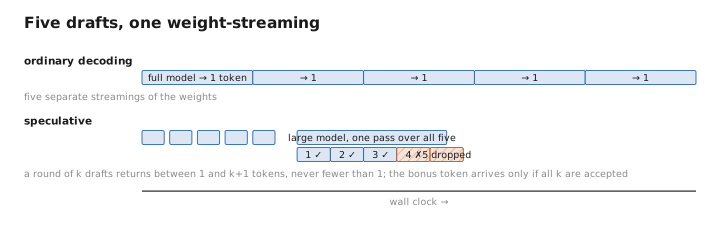
Figure 1. Five drafts, one weight-streaming.
A pinch of math: why the output is identical
The acceptance rule is the part that matters, because a careless rule would bias the output toward whatever the draft model likes.
Let $p$ be the large model’s probability for a token and $q$ the draft model’s, both at the same position. The draft proposed a token $x$ sampled from $q$. Accept it with probability
$$\min\!\left(1, \frac{p(x)}{q(x)}\right)$$So if the large model considers the token at least as likely as the draft did, accept unconditionally. If the large model considers it less likely — the draft over-proposed — accept with probability equal to the ratio, which is the fraction of the proposal the large model endorses.
On rejection, do not simply resample from $p$; that would over-represent tokens the draft already had a chance to propose. Instead sample from the residual:
$$p'(x) = \frac{\max\big(0,\; p(x) - q(x)\big)}{\sum_{x'} \max\big(0,\; p(x') - q(x')\big)}$$This is the part of the large model’s distribution that the draft failed to cover, renormalized. Tokens the draft over-proposed are zeroed out, having already had their fair share of chances; tokens the draft under-proposed absorb the whole shortfall.
Put the two together and every token ends up drawn from exactly $p$. The argument is short enough to sketch: a token can emerge either by being proposed and accepted, which happens with probability $q(x) \cdot \min(1, p(x)/q(x)) = \min(q(x), p(x))$, or by being drawn from the residual after some rejection. Summing the two contributions gives $p(x)$ exactly, for every token.
This is rejection sampling, and the guarantee is not statistical or approximate. The sequence produced is drawn from the identical distribution the large model alone would have produced. Run it at temperature zero and you get the same tokens the large model would have produced, deterministically. There is no quality trade to evaluate, which is unusual enough in this field to be worth stating twice.
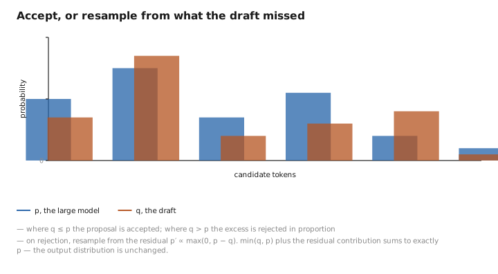
Figure 2. Accept, or resample from what the draft missed.
What determines the speedup
Two quantities, pulling against each other.
The acceptance rate is how often a drafted token survives, and it is set by how well the draft model imitates the large one. It is not uniform across text: highly predictable stretches — boilerplate, closing brackets, the second half of a common word, formulaic phrasing — are accepted at very high rates, while genuinely uncertain positions are rejected often. In effect the technique runs fast through the easy parts of a response and falls back to ordinary speed at the hard parts, which is a reasonable allocation.
The draft length trades expected gain against expected waste. Longer drafts offer more tokens per verification, but acceptance is multiplicative — the expected number accepted from a draft of $k$ tokens at per-token acceptance $\alpha$ is roughly $(1 - \alpha^{k+1})/(1 - \alpha)$, which saturates. Beyond a handful of tokens you are mostly generating drafts that will be thrown away. In practice four to eight is typical, and the best implementations adapt it, drafting further when recent acceptance has been high.
Realistic end-to-end speedups are two to three times. Not the five or eight that the draft length might suggest, because the drafting itself costs something and rejections waste work, but a substantial and free improvement.
Removing the second model
Maintaining a separate draft model is an operational nuisance — another checkpoint to train, store, load, and keep aligned with the target as it is updated. Several variants avoid it.
Self-speculation uses the large model as its own draft by running only a subset of its layers, on the observation from the logit lens that a partial forward pass already produces a usable prediction. The draft costs a fraction of a full pass and needs no separate model.
Multi-token prediction trains the model with extra output heads that predict two, three, or four positions ahead, so a single pass yields both the next token and a draft of what follows. The heads are cheap, and there is evidence that training this way improves the model’s ordinary quality as well, since predicting further ahead is a harder objective that seems to encourage better planning. Some recent large models ship with such a head specifically to make speculation available at serving time.
Retrieval-based drafting dispenses with neural prediction entirely and proposes continuations copied from the prompt or from a cache of recent text. This sounds crude and works remarkably well for the tasks where copying is what is wanted — editing a document, answering from a supplied passage, regenerating code with a small change — because in those settings long stretches of the output genuinely are verbatim from the input, and a lookup accepts where a small model would have had to guess.
Where it helps and where it does not
One important limitation, which follows directly from the mechanism.
The technique converts idle arithmetic into tokens, and it therefore requires that arithmetic to be idle. At small batch sizes it is: one sequence at a time leaves the chip almost entirely unoccupied. But as the article on KV cache explained, batching also converts idle arithmetic into throughput, by amortizing the weight reads across many sequences. A server running a large batch has already spent the surplus, and speculation then competes for the same resource rather than exploiting a free one — the extra work of verifying rejected drafts becomes a genuine cost, and the speedup shrinks or disappears.
So the two techniques address the same slack from different directions and do not compose well. Speculation is for latency: a single user waiting on a single response, where batching cannot help because there is nothing to batch. Batching is for throughput: many users at once, where per-request latency matters less than aggregate cost. Serving systems accordingly enable speculation for interactive low-concurrency traffic and disable it under load, which is the correct reading of a mechanism that exists to spend something that is only sometimes free.
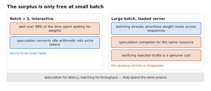
Figure 3. The surplus is only free at small batch.
What to carry forward
Speculative decoding produces text drawn from exactly the distribution the large model would have produced, several times faster, by exploiting the fact that generation is limited by the bandwidth needed to stream weights rather than by arithmetic — so checking five candidate tokens costs a single weight-streaming, nearly the same as generating one. A small draft model proposes a short continuation, the large model verifies the whole draft in one pass, and the longest surviving prefix is kept. Exactness comes from the acceptance rule: accept a proposal with probability equal to the ratio of the large model’s probability to the draft’s, capped at one, and on rejection resample from the residual distribution — the part of the large model’s beliefs the draft failed to cover, with over-proposed tokens zeroed out. Together these make every emitted token a draw from the target distribution, so there is no quality trade to weigh. The speedup depends on the acceptance rate, which is high on predictable stretches and low on genuinely uncertain ones, and on the draft length, whose returns saturate because acceptance compounds multiplicatively; two to three times is typical. The separate draft model can be dispensed with by running a subset of the large model’s own layers, by training extra heads that predict several positions ahead, or by copying candidate continuations from the prompt — the last being unexpectedly effective wherever the output is largely verbatim from the input. And the whole technique depends on the arithmetic being idle, so it helps a single user waiting on a response and stops helping a heavily batched server, which has already spent that surplus on throughput.
The figures in this article follow the shared figure key , which explains what every shape, line style and colour means.
