The article on attention opened by dismissing the running summary: a fixed-size vector, updated word by word, that must hold everything worth knowing about a sequence and inevitably crowds out the distant past. Attention replaced it with direct access to every position, and the field never looked back. Except that the running summary had one property attention gave up, and after a decade of paying for it, the property became worth revisiting. A model that carries a fixed-size state does not have a KV cache that grows without limit, and does not cost more per token as the conversation lengthens. It is also, as the article on linear attention shows, where you arrive if you start from attention and simplify rather than starting from recurrence and repairing. This piece is about what it took to make the running summary competitive again, what it still cannot do, and why the answer that is winning is neither one thing nor the other.
The trade, stated plainly
Attention keeps everything. To generate a token it consults every previous position, exactly, which means the past is available in full detail and the cost of the consultation grows with how much past there is. Memory grows linearly with length, and time per token grows linearly too, since the cache must be scanned.
A recurrent model keeps a summary. To generate a token it consults a fixed-size state, which is updated by each new token and never grows. Memory per sequence is constant. Time per token is constant. And whatever did not fit in the state is gone, irrecoverably, because nothing was stored to go back to.
Neither is strictly better. Attention buys perfect recall with unbounded cost; recurrence buys bounded cost with lossy memory. What made attention win was not that the trade favoured it in principle, but two practical facts: the old recurrent models could not be trained in parallel, since the state at position ten requires the state at position nine, so a sequence had to be processed one step at a time; and their memory was too lossy to be useful at any interesting length. The modern work fixed the first and improved the second.
Making a recurrence trainable in parallel
The starting point is a linear recurrence — a state updated by a matrix multiplication and an input, with no nonlinearity in the update itself:
$$h_t = A h_{t-1} + B x_t, \qquad y_t = C h_t$$Linearity is the crucial restriction, and it is what buys back parallelism. Unroll the recurrence and the state at any position is a weighted sum over all previous inputs:
$$h_t = \sum_{k=0}^{t} A^{k} B\, x_{t-k}$$which is a convolution of the input sequence with a kernel built from powers of $A$. And a convolution can be computed for all positions at once, in parallel, without stepping through the sequence. So the model has two forms: a convolution during training, where the whole sequence is present and parallelism is what matters, and a recurrence during generation, where tokens arrive one at a time and constant-cost updating is what matters. Same parameters, same function, two schedules — which is the property that made the whole line of work viable.
Making it work, rather than merely run, required getting $A$ right. A randomly chosen matrix either forgets almost immediately or blows up, since everything depends on powers of it. The breakthrough was to initialize $A$ from a particular structured family, derived from the classical problem of approximating a function by its projection onto orthogonal polynomials, whose powers decay in a graded way so that the state retains a compressed record of the whole history at multiple timescales rather than only the recent past. That is what lifted these models from a curiosity to something that could model long sequences at all.
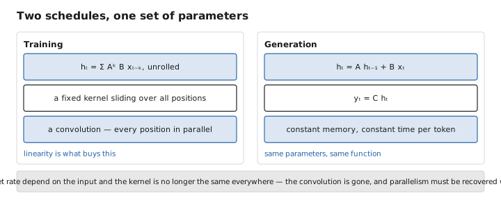
Figure 1. Two schedules, one set of parameters.
The missing ingredient: selectivity
Even with a good $A$, one problem remained, and it is the one that separates the successful designs from their predecessors.
In the recurrence above, $A$, $B$, and $C$ are fixed. The same update is applied regardless of what the token is. The model compresses history at a rate it decided once, in advance, and cannot decide to remember this token and forget that one. Attention, by contrast, is content-dependent by construction — the whole mechanism is a comparison that decides what to look at based on what is there.
The fix is to make the recurrence’s parameters functions of the input: let $B$, $C$, and the forgetting rate be computed from the current token rather than fixed. Now the model can hold a state open for something important and let it decay for filler, which is precisely the capability a fixed recurrence lacks. On the toy task that exposes this — copy a specific token from far back in the sequence while ignoring everything between — a fixed recurrence fails and a selective one succeeds.
This is the idea behind the Mamba family, and it comes at a price. Making the parameters input-dependent destroys the convolution, because a convolution requires a kernel that is the same everywhere and there is no longer one. Parallelism has to be recovered a different way, by an associative scan — an algorithm that computes all the prefix states of an associative operation in logarithmic depth rather than linear, the same technique used for parallel prefix sums. Combined with an implementation that keeps the state in fast memory and never writes intermediate states to slow memory, in exactly the spirit of FlashAttention , this is fast enough in practice.
What a fixed state cannot do
The honest limitation follows from the definition and no amount of engineering removes it.
A fixed-size state can hold a fixed amount of information. If a task requires reproducing something from a hundred thousand tokens back, verbatim, and the state is a few thousand numbers, the information must have been discarded unless the model somehow knew at the time that it would be needed. Attention has no such problem, because it kept everything.
The tasks that expose this are precisely the ones that matter in practice. Retrieving a specific fact from a long document. Following a chain of references. Copying a long string. In-context learning from many examples, which depends on the induction mechanism of finding an earlier occurrence and reading off what followed — an operation that requires the earlier occurrence to still be available in full, which is exactly what a compressed state does not guarantee.
Measured on language modelling loss, selective state space models match transformers of the same size. Measured on retrieval from long contexts, they do noticeably worse. Both facts are true simultaneously, and the reason they are compatible is that average next-token prediction is dominated by local structure, where a summary is entirely adequate, while retrieval is a small fraction of tokens where a summary is fatal. This is a good illustration of the evaluation point that a headline metric can be matched while a specific capability is not.
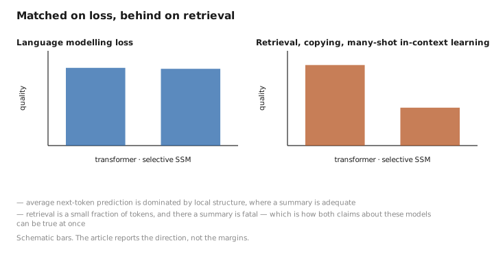
Figure 2. Matched on loss, behind on retrieval.
Hybrids, and where this has landed
The resolution the field has reached is not to choose. Interleave the two: mostly recurrent layers, with a small proportion of full attention layers distributed through the stack — commonly one in six or one in eight.
The reasoning is that recall does not need to be available at every layer. A few attention layers give the model somewhere to perform exact lookups when it needs them, while the recurrent majority handles the bulk of the processing at constant cost per token. In practice such hybrids match or exceed pure transformers on general quality, retain most of their retrieval ability, and carry a cache a small fraction of the size — since only the attention layers need one.
This has moved from research to production. Several current models of significant size use this arrangement, and it is the most credible answer available to the problem the article on long context describes: a cache that grows forever is the binding constraint on serving, and the only structural fix is for most layers not to have one.
The broader lesson is worth stating, because it recurs. The running summary was not wrong; it was untrainable in parallel and too lossy, and both were fixable. What it offered — bounded state — was a genuine advantage that the field spent a decade paying to do without, and the eventual answer was not that one mechanism replaced the other but that the two do different jobs and a model can have both.
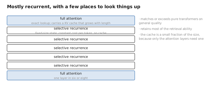
Figure 3. Mostly recurrent, with a few places to look things up.
What to carry forward
A state space model carries a fixed-size summary of everything it has read, updated token by token, so its memory does not grow with the sequence and its cost per token is constant — the property attention gave up when it chose perfect recall at unbounded cost. What made the older recurrent models unusable was that they could not be trained in parallel, and the fix is linearity: a linear recurrence unrolls into a convolution, which computes every position at once, so the same parameters run as a convolution during training and as a recurrence during generation. Making it work also required the state-update matrix to be initialized from a structured family whose powers decay in a graded way, retaining a compressed record at multiple timescales rather than only the recent past. The remaining gap was selectivity — a fixed recurrence applies the same update to every token and cannot decide to remember one thing and forget another — closed by making the recurrence’s parameters functions of the input, at the cost of destroying the convolution and requiring an associative scan to recover parallelism. What no amount of engineering fixes is that a fixed state holds fixed information: these models match transformers on language modelling loss and fall behind on retrieval from long contexts, in-context learning from many examples, and anything requiring an earlier occurrence to be recovered exactly. The field’s answer has been to interleave — mostly recurrent layers with roughly one attention layer in six or eight — which retains most of the recall, matches transformer quality, and shrinks the cache to a small fraction, since only the attention layers need one.
The figures in this article follow the shared figure key , which explains what every shape, line style and colour means.
