There is a familiar experience with a hard question. The model answers, the answer is wrong, you paste the identical prompt back in, and the second answer is right. Nothing changed. What happened is that a language model does not hold an answer, it holds a distribution over answers, and the reply on the screen is one draw from it. On a hard question it is spread across candidates, one of them correct, and the reply you were shown was the unlucky sample. Industrialized, that observation becomes the family of techniques filed under test-time compute: buying accuracy with extra forward passes when the question is asked rather than extra parameters when the model is built. This piece is about how the buying is done, what the price schedule looks like, and where the purchase stops working.
Accuracy left on the table, and who pays to collect it
A trained model holds a conditional distribution over continuations, and every reply is one sample from it, drawn under whatever decoding policy the surrounding software uses. On a hard problem that distribution is broad: the correct answer sits inside it at modest probability — a fifth of the mass, a twentieth, sometimes less — among plausible neighbours wrong in different ways. So the accuracy a model appears to have, measured one sample at a time, is lower than the accuracy its distribution contains. That gap is measurable, and recoverable. Not for free.
The framing that makes this interesting is not the accuracy but where the cost falls. Training compute is spent once, in advance, by whoever built the model; inference compute is spent per request, forever, by whoever is asking. A technique that turns one forward pass into thirty-two moves expenditure across that boundary, converting a fixed cost borne by the provider into a variable one borne on every query. That is a change in the economics, not only in the score. The scaling laws that governed the field’s spending describe the first budget and are silent on the second.
The multiple is less brutal than it looks, which is why anyone bothers. Samples of one prompt share a prefix and run together, so continuous batching keeps the wall-clock penalty well below the raw multiple. The arithmetic is billed regardless.
Sampling several times and taking the most common
The cheapest way to spend the extra passes is the obvious one: draw several answers at a temperature high enough that they differ, extract the final answer from each, and return whichever value appears most often. This is self-consistency, or plainly majority voting, and it needs nothing beyond an equality test.
It works because of two asymmetries pointing the same way. A chain of reasoning can go wrong in a great many ways, so errors scatter across distinct wrong answers; a chain that goes right has nowhere to arrive except the one correct answer, so successes pile up on a single value. Diverse errors, coincident successes. A plurality therefore lands on the correct answer well before any individual sample reliably finds it, and can be right when most samples were wrong. Asking three strangers for directions and going with the two who agree is the same instinct, and fails the same way.
It requires an answer comparable for equality. That confines it to a short canonical form — a number, a label, a choice from a menu — and excludes essays, explanations, and code, where two correct responses differ in every token. Patches exist: cluster by semantic similarity, or ask a model whether two answers agree. Each reintroduces the judgement the plain method was valuable for not needing.
It fails silently when the model is confidently and consistently wrong. A plurality of identical errors looks exactly like agreement, because it is agreement; voting measures consensus, and consensus is evidence of correctness only when the errors are independent. Where a misconception is stable across samples — a misread constraint, a formula remembered wrongly — the vote returns the same wrong answer with more apparent confidence, and the disagreement that might have flagged it is averaged away.
The gain flattens quickly. Most of the improvement arrives in the first handful of samples, well before the counts people quote, which matters for reading results as much as for spending money: a figure obtained with sixty-four votes is not comparable to a single-sample figure from another system, as the article on evaluation insists at greater length. The distinction gets dropped routinely.
Best-of-n needs something that can rank
The dividing line in this family is whether an external signal is available. Majority voting needs none, which is its appeal. Best-of-$n$ needs something that can rank a set of candidates, and the method’s behaviour follows entirely from what that something is.
Where a real checker exists, the ranking is sound and the method is strong. A test suite runs the candidates and keeps one that passes; a proof checker accepts a proof or does not. These are the same verifiers that make reinforcement learning from verifiable rewards possible — the reward is a fact, not an estimate, so selecting the maximum really is selecting the best. The cost is the checker’s narrowness, not its honesty: give a coding problem three weak tests and best-of-$n$ returns the candidate that special-cases them.
Where no checker exists, the ranker is a learned reward model , and the method inherits every pathology of one. The sharpest is definitional: drawing many candidates and returning the highest-scoring one is a well-funded search for whatever the ranker has got wrong. A single sample tests a reward model fairly. The maximum of a hundred tests it adversarially, using the generator’s diversity to find the corners where its scores are high and its judgement poor.
So increasing $n$ eventually makes results worse. This is not a subtlety and not a bug in anyone’s implementation but the expected behaviour of maximizing a proxy, and the standard remedies — penalizing distance from the base distribution, capping $n$, ensembling rankers — amount to declining to optimize too hard rather than to fixing the proxy.
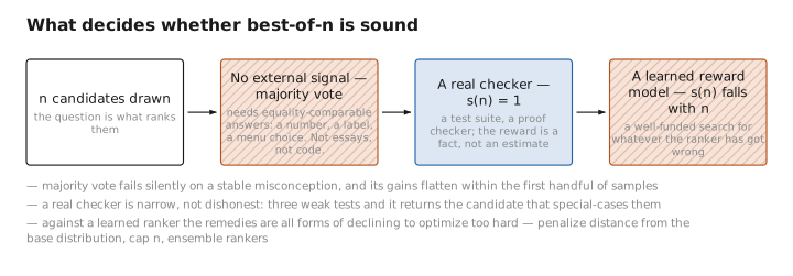
Figure 1. What decides whether best-of-n is sound.
Depth is not the same purchase as coverage
A final-answer verifier says nothing until the answer exists, so a doomed attempt is paid for in full before anything notices. Scoring intermediate steps gives a signal early enough to act on.
Process rewards buy a denser signal at the price of a far more expensive label. A model trained to score partial solutions can guide a search over prefixes, expanding the promising and abandoning the rest, which is more sample-efficient than generating whole attempts and throwing most away. What it needs is step-level supervision, costly to collect and a judgement in a way the final answer is not — whether the fourth line of a derivation was a good move is arguable, whether the final number matches is not.
Tree search over reasoning steps works in constrained domains and has been hard to make pay off in open-ended ones. Where the state is checkable and the branching means something — formal proof, board games, tightly specified puzzles — searching over partial solutions is established practice. Where it is not, the search spends its budget distinguishing prefixes the scorer cannot really distinguish, and gains over sampling more whole attempts have been modest.
Letting one attempt think for longer is not the same as taking many short attempts. The first buys depth, the second coverage, and they fail differently. A single long chain, of the kind a reasoning model produces, can commit to an error in its third step and spend four thousand tokens elaborating it into something detailed and self-consistent, the length supplying confidence rather than correction. Many short attempts cannot do that, and cannot reach an answer needing ten steps of setup — every sample fails in the same place, and width is no substitute for depth.
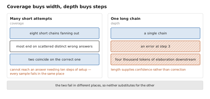
Figure 2. Coverage buys width, depth buys steps.
A pinch of math: coverage against selection
Two quantities are in play, and conflating them is the standard error. Let $p$ be the probability that a single sample is correct. Then coverage, the probability that at least one of $n$ samples is correct, is
$$\text{cov}(n) = 1 - (1-p)^n$$which rises steeply and then saturates. With $p = 0.2$, one sample is right one time in five, while $n = 8$ gives coverage of about $0.83$ and $n = 32$ about $0.999$. The correct answer is almost certainly in the pile. That is the optimistic curve, and the one usually plotted.
The achieved accuracy is not that curve. It is that curve multiplied by the probability that whatever mechanism you use actually returns a correct candidate from the pile:
$$\text{acc}(n) = \big(1 - (1-p)^n\big) \cdot s(n)$$where $s(n)$ is the selector’s reliability. Majority voting is one choice of $s$, best-of-$n$ with a checker another, with a learned ranker a third. Given a sound checker, $s(n) = 1$ and accuracy simply is coverage, which is why verifiable domains produce the headline results. Given an imperfect selector, $s(n)$ falls as $n$ grows, since a larger pile holds more high-scoring wrong candidates, and the product can decline while coverage climbs. Two curves moving in opposite directions. The gap between them is where this subject lives.
Saturation also explains the deflationary part. Reported gains run roughly linearly in $\log n$, so each doubling of the sample count buys a constant and then a shrinking increment, and whether that trade beats training a larger model has no clean answer: it depends on the task, on whether a checker exists, and above all on how often the question will be asked, since inference cost recurs and training cost does not. A hundred forward passes per query is not obviously cheaper than a bigger model, and at high volume it is obviously not. Sampling once and training on the winners — distillation of a search into a policy — converts the recurring cost into a one-off, and inherits the ceiling of what the search reached.
Which is the last thing the formula says. If $p = 0$, then $\text{cov}(n) = 0$ for every $n$.
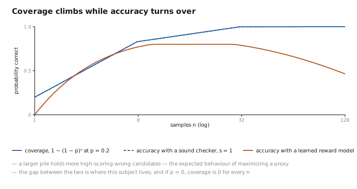
Figure 3. Coverage climbs while accuracy turns over.
What to carry forward
A single reply is one draw from a distribution, and on hard problems that distribution frequently contains a correct answer the draw missed, so accuracy can be bought back with extra forward passes at the moment of asking rather than extra parameters at build time — which shifts cost from the provider’s one-off training bill to the asker’s recurring one, a change in economics and not only in scores. The cheapest method, sampling several answers and returning the most common, works because errors scatter while correct answers coincide; it needs no external signal, and pays with three restrictions — it wants an answer comparable for equality, so essays and code are out; it fails silently when a stable misconception makes every sample agree; and its gains flatten early, which makes a figure quoted at sixty-four votes incomparable to a single-sample one. Best-of-$n$ replaces the vote with a ranker, and everything turns on what the ranker is: a test suite or proof checker makes the selection sound, while a learned reward model turns drawing candidates and taking the maximum into an efficient search for the ranker’s own mistakes, so results eventually degrade as the count rises — the expected behaviour of maximizing a proxy. Scoring intermediate steps gives a denser signal that can guide a search over partial solutions, at the price of step-level labels that are expensive and themselves a judgement, and that search has paid off in constrained domains more than open-ended ones. Thinking longer buys depth, sampling more buys coverage, neither substitutes for the other. Under all of it sits one limit: coverage is one minus the miss rate raised to the sample count, so when the miss rate is one, no count helps. These methods amplify what the distribution already reaches rather than extending its reach.
The figures in this article follow the shared figure key , which explains what every shape, line style and colour means.
