Before a model sees anything, text has to be cut into pieces and each piece assigned a number. This is the only step in the entire pipeline that does not learn. The embedding table is trained, the attention weights are trained, the output map is trained; the tokenizer is a fixed recipe, built once from a sample of text by an algorithm with no notion of meaning, and thereafter frozen. Everything the model can express is expressed in units this recipe chose, and a surprising number of the odd behaviours people notice — trouble with arithmetic, trouble counting letters, uneven costs across languages, occasional total derangement on a particular string — trace back to it. This piece is about how the pieces are chosen and what the choice costs.
The two obvious approaches, and why neither works
Start with words. Split on spaces and punctuation, assign each distinct word a number, and you have a vocabulary that matches how people think about language. It fails in three ways at once. The vocabulary is unbounded, since new words appear constantly and proper nouns are effectively infinite; anything not in the list must be replaced by a single “unknown” symbol, which destroys the information entirely; and the relationship between run, runs, running, and runner is invisible, because four unrelated numbers say nothing about their common root. Languages that build words by agglutination, where a single word carries what English needs a clause for, are hurt worst of all.
Now try characters. The vocabulary is small and closed, nothing is ever unknown, and morphology is at least visible in principle. But sequences become enormously long — a page of English is several thousand characters — and since attention costs grow with the square of the length, the model spends its budget on a stream of individual letters. Worse, almost all of that work is spent rediscovering that t-h-e is a unit, in every context, forever. The model is made to learn the alphabet before it can learn anything else.
The compromise is subword tokenization: a fixed vocabulary of a few tens of thousands of pieces, where common words are single tokens, rare words are assembled from fragments, and no input is ever unrepresentable because the individual characters remain in the vocabulary as a fallback. Frequency decides the granularity. “The” is one token; an unusual surname might be five.
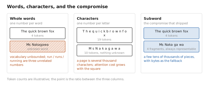
Figure 1. Words, characters, and the compromise.
How the pieces get chosen
The dominant method is byte pair encoding, borrowed from a data-compression algorithm from the 1990s, and its logic is almost embarrassingly simple.
Begin with a vocabulary of individual bytes, so that any possible input is representable. Take a large corpus and count every adjacent pair of symbols in it. Find the pair that occurs most often — say t followed by h — and add th to the vocabulary as a new symbol, replacing every occurrence. Count again. Merge again. Repeat until the vocabulary reaches the size you wanted.
That is the whole algorithm. What it produces, after fifty thousand merges, is a vocabulary in which frequently co-occurring sequences have been glued into units. Nobody supplies linguistic knowledge; the merges discover that ing and tion are worth having because those letters keep turning up together, not because anyone told the algorithm about suffixes. The result frequently resembles morphology and is not morphology, which is the source of much of what follows.
The merge list is ordered, and applying the tokenizer to new text means replaying those merges in the same order. This makes tokenization deterministic and fast, and it also means the tokenizer’s behaviour is entirely determined by the corpus it was built from. A tokenizer trained mostly on English will represent English efficiently and everything else badly.
Two details of practice matter. Text is usually pre-split on a pattern before merging, so that merges cannot cross word boundaries or absorb spaces in unhelpful ways. And the leading space is conventionally attached to the following word, so that " cat" and "cat" are different tokens — which is why models sometimes behave differently depending on whether your prompt ends with a space, and why a trailing space in a prompt is a small but real way to confuse a model.
What the choice costs
Several well-known model failures are tokenizer failures, and it is worth going through them because in each case the model is being blamed for something it was never given the means to do.
Counting letters. Ask a model how many times the letter r appears in a word and it may well get it wrong. The reason is that it never received the letters. It received two or three tokens, each an opaque index into a table, and the spelling of a token is not information the model has access to except insofar as it has memorized it from text discussing spelling. Asking a model to count letters is asking it to report on something below its perceptual floor. That models do it as often as they do is the surprising part.
Arithmetic. Numbers tokenize badly and inconsistently. Depending on the vocabulary, 1234 may be one token, or 12 and 34, or 1, 23, 4 — and crucially the grouping depends on the digits, so 1235 may split differently from 1234. Any algorithm for addition has to work on digits aligned by place value, and a model whose inputs are irregularly grouped chunks has to learn place-value arithmetic separately for every grouping pattern. The most effective fix has been the crudest: force every digit to be its own token. Several recent models do this, and their arithmetic improves accordingly.
Cost and fairness across languages. A tokenizer built mostly from English text represents English in roughly four characters per token. The same tokenizer may need two or three times as many tokens for the same content in another language, and considerably more for scripts poorly represented in the training corpus. Since the context window is counted in tokens and billing is per token, the identical document costs several times more to process in one language than another, and fits into a proportionally smaller share of the window. This is a straightforward inequity that follows entirely from whose text was in the corpus.
Glitch tokens. Occasionally a token exists in the vocabulary but appears almost never in the training data — an artifact of the tokenizer being built on a different corpus, or a wider one, than the model was subsequently trained on. Its embedding row is therefore close to its random initialization, since the gradient described in that article only ever reaches rows the batch contained. Feed such a token to a model and it behaves erratically: refusing to repeat it, substituting a different word, producing nonsense. These are the strings people collect and trade as curiosities, and their explanation is mundane — the model is being shown a vector it never learned anything about.
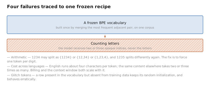
Figure 3. Four failures traced to one frozen recipe.
A pinch of math: what vocabulary size buys and costs
The size of the vocabulary is a real design decision with a trade on each side, and it can be reasoned about directly.
Larger vocabularies compress better. Each token carries more characters on average, so a document becomes fewer tokens, which reduces both the cost of attention and the length of the KV cache . If $c$ is the average characters per token, the attention cost for a document of $C$ characters falls with $(C/c)^2$ — so improving compression by a quarter removes roughly a third of the attention work.
But the embedding and output matrices scale directly with vocabulary size $V$:
$$\text{parameters in the two maps} = 2 \times V \times d_{\text{model}}$$At $V = 128{,}000$ and $d = 4096$, that is over a billion parameters spent on the vocabulary alone, plus the cost of computing a logit for every entry at every position. And there is a subtler cost: with a fixed corpus, doubling the vocabulary halves the average number of times each token is seen, so each embedding row gets less training. The tail of a large vocabulary is under-trained by construction, which is the same mechanism that produces glitch tokens.
The balance has shifted upward over time. Early models used around thirty thousand tokens; current ones commonly use a hundred thousand or more. The reason is that models grew faster than vocabularies needed to, so the fixed cost of the two maps became a smaller share of the whole — while the compression benefit, which multiplies against the ever-growing context length, became more valuable. Multilingual coverage pushes the same way, since serving many languages fairly requires vocabulary space for all of them.
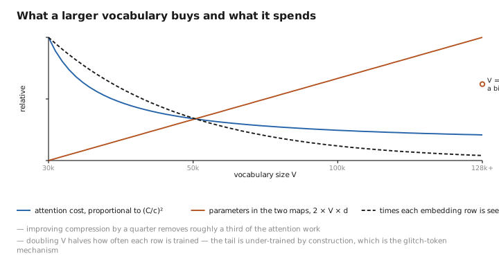
Figure 2. What a larger vocabulary buys and what it spends.
Living with it, and living without it
Because the tokenizer is frozen before training, changing it means retraining, and this rigidity has consequences. A model cannot be extended to a new script after the fact without surgery on the embedding table. Two models with different tokenizers cannot straightforwardly share distilled outputs, since their vocabularies do not align — a real obstacle for distillation across model families, and one that has produced a small literature on aligning mismatched tokenizers.
The obvious question is whether the step can be removed. Byte-level models that consume raw bytes and learn their own grouping have been built repeatedly, and they solve every problem listed above at once: no unknown tokens, no script bias, no glitch tokens, spelling fully visible, arithmetic on plain digits. The cost is sequence length, and the research programme has been about recovering it — typically by having a small network group bytes into patches dynamically, spending most of the model’s depth on the patches and only a little on the bytes. Recent work in this direction is genuinely promising, allocating more compute to unpredictable stretches of text and less to predictable ones, which is something a fixed vocabulary cannot do. Whether it displaces subword tokenization is unsettled, though the same question arises for images, where a patch grid plays exactly this role and imposes exactly this kind of floor. What is clear is that the current arrangement is a compromise made for tractability, that it is the source of a specific and well-understood set of failures, and that nobody defends it as correct.
What to carry forward
Tokenization is the one step in the pipeline that does not learn: a fixed recipe, built once by counting, that decides the units in which everything downstream must be expressed. Whole words give an unbounded vocabulary and no way to relate related forms; individual characters give sequences so long that quadratic attention costs become prohibitive; subword pieces are the compromise, with common words as single tokens and rare ones assembled from fragments. The standard construction, byte pair encoding, repeatedly merges the most frequent adjacent pair until the vocabulary is full — a compression algorithm with no linguistic knowledge, which produces something that resembles morphology without being it. The failures that follow are specific and explicable: models cannot count letters because they never receive letters; arithmetic suffers because digits group irregularly and inconsistently, which is why forcing one token per digit helps; text in under-represented languages costs several times more tokens for the same content, in both money and context; and glitch tokens misbehave because their embedding rows, never having appeared in training, remain close to random initialization. Vocabulary size trades compression — which reduces attention cost and cache size quadratically and linearly — against a billion or more parameters in the two maps and a tail of rows that each get proportionally less training. And because the tokenizer is frozen before training begins, the whole arrangement is difficult to change afterwards, which is why byte-level models that learn their own grouping remain an active and plausible line of attack on the entire problem.
The figures in this article follow the shared figure key , which explains what every shape, line style and colour means.
