Lesson 1 — The Big Picture: What Is a Diffusion Model?

Course map. Ten lessons. We start from intuition, build the forward (noising) process, derive the reverse (denoising) process from the variational lower bound, collapse it into the famous one-line training loss, study the network that implements it, write the training loop, then the sampling loop, then the fast/deterministic samplers and the score-based view, and finally conditioning, guidance and latent diffusion. Each lesson opens with a recap of the previous one and closes with a conclusion.

Course map and prerequisites. The full ten-lesson table of contents, the suggested reading order, and a prerequisites list (what background to have before starting, and where each piece is first needed) live in the Course Index . The complete symbol glossary is in Appendix B ; acronyms are in Appendix A . This lesson assumes only comfort with deep learning; the probability machinery enters in Lessons 2–4.

---

Destruction is the easy art. A photograph left in the sun fades; a struck match burns down to nothing; a clear radio signal dissolves into hiss. None of it takes talent. The strange, almost suspicious feat would be to run any of these backwards — to coax a sharp image out of a fog of static, one careful step at a time, and have it emerge not as the original but as something wholly new and equally convincing. A diffusion model is a machine built to perform exactly that feat. This first lesson is the view from altitude, before we descend into the gears.

Overview

Imagine a sharp photograph that you corrupt by sprinkling sand on it, a little at a time. After one handful you can still see the picture; after a hundred it is structureless sand. This destruction is easy: anyone can pour sand. The hard, magical part is the reverse — removing exactly one handful and recovering the slightly cleaner image underneath. If you could do that one tiny step reliably, you could start from pure sand and, by repeating the small reversal, conjure a brand-new sharp photograph that never existed.

That is the entire idea:

1. Forward process (training-time only): take real data and gradually corrupt it with Gaussian noise until it becomes (approximately) $\mathcal N(0,I)$. This direction is fixed, has no learnable parameters, and is trivial to evaluate.
2. Reverse process (the learned model): train a neural network to undo one small step of corruption. At inference we start from $x_T\sim\mathcal N(0,I)$ and apply this learned denoiser many times until a clean $x_0$ emerges.

The asymmetry is the whole trick. Adding noise is free; removing it is what we learn. Because each step removes only a tiny amount of noise, the conditional it must model is gentle and (as we will show in Lesson 3) close to Gaussian — which is precisely why diffusion models train stably and sample at high quality.

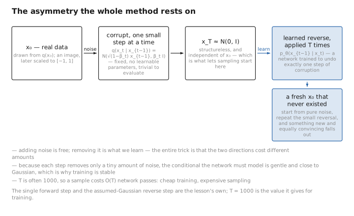
Figure 1. The asymmetry the whole method rests on.

Where this sits in the generative-model landscape

Before we touch a single equation, it helps to know what kind of animal we are dealing with — and the quickest way to know an animal is to stand it beside its relatives.

Generative modeling means learning $p_\theta(x)$ that approximates the true data law $q(x)$ so we can draw novel $x\sim p_\theta$. Families differ along three axes: likelihood tractability (can we evaluate or bound $\log p_\theta(x)$?), sampling cost (how many network evaluations per sample?), and training stability (is the objective a well-posed optimization, or a min–max/adversarial one?).

Family	Likelihood	Sampling cost	Training	Failure mode
GAN	none (implicit)	1 forward pass (fast)	min–max game	non-convergence, mode collapse
VAE	ELBO lower bound	1 forward pass (fast)	single max-likelihood bound (stable)	blurry samples, posterior collapse
Autoregressive	exact $\log p_\theta$	$O(\dim x)$ sequential (slow)	exact MLE (stable)	slow sampling, ordering bias
Normalizing flow	exact $\log p_\theta$	1 pass (fast)	exact MLE (stable)	constrained invertible architectures; expensive Jacobians
Diffusion	ELBO lower bound	$O(T)$ passes (slow; $T$ up to $10^3$)	regression / ELBO (very stable)	slow sampling (mitigated by DDIM, distillation)

A few points sharpened:

• GANs optimize $\min_\theta\max_\phi V(\theta,\phi)$; sampling is a single generator pass, but there is no explicit density and the saddle-point objective is delicate (Goodfellow et al., 2014).
• VAEs maximize the ELBO $\mathbb E_{q_\phi(z\mid x)}[\log p_\theta(x\mid z)] - \mathrm{KL}(q_\phi(z\mid x)\,\|\,p(z))$ jointly over encoder $q_\phi$ and decoder $p_\theta$ (Kingma & Welling, 2014).
• Autoregressive models give exact likelihood via $p(x)=\prod_i p(x_i\mid x_{\lt i})$ but require $O(\dim x)$ sequential evaluations to sample.
• Normalizing flows use invertible $f_\theta$ with $\log p_\theta(x)=\log p(z)+\log|\det \partial f_\theta/\partial x|$; exact likelihood at the cost of architectural invertibility and tractable log-determinants (Rezende & Mohamed, 2015).
• Diffusion turns generation into many small denoising steps; the objective is a stable regression (Sohl-Dickstein et al., 2015; Ho et al., 2020), at the cost of $O(T)$ network evaluations per sample.

Diffusion as a hierarchical VAE with a fixed encoder

The latent-variable view makes the “deeply hierarchical VAE” claim precise. A diffusion model defines a joint over data $x_0$ and a chain of latents $x_{1:T}$:

$$ p_\theta(x_{0:T}) = p(x_T)\prod_{t=1}^{T} p_\theta(x_{t-1}\mid x_t), \qquad p(x_T)=\mathcal N(0,I). $$

A standard VAE has an encoder $q_\phi(z\mid x)$ and a decoder $p_\theta(x\mid z)$, trained jointly. A diffusion model is the special case of a $T$-level hierarchical VAE with latents $z=(x_1,\dots,x_T)$ in which the inference network is not learned but fixed to the forward chain

$$ q(x_{1:T}\mid x_0)=\prod_{t=1}^T q(x_t\mid x_{t-1}), \qquad q(x_t\mid x_{t-1})=\mathcal N\!\big(\sqrt{1-\beta_t}\,x_{t-1},\,\beta_t I\big). $$

Because $q$ has no parameters $\phi$, only the decoder chain $p_\theta(x_{t-1}\mid x_t)$ is learned. The training objective is the same ELBO as a VAE — maximize a lower bound on $\log p_\theta(x_0)$ — and reduces, term by term, to making the learned reverse $p_\theta$ match the true reverse of the fixed $q$. We derive that ELBO and its per-step decomposition in Lesson 4.

Remark (why fix the encoder?). Freezing $q$ removes the encoder-posterior optimization that makes hierarchical VAEs hard to train, and it gives the forward marginals $q(x_t\mid x_0)$ in closed form (Lesson 2). The price is that the latents share the dimensionality of the data and the chain is long, hence the $O(T)$ sampling cost.

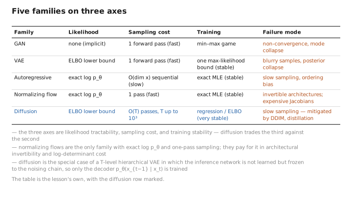
Figure 2. Five families on three axes.

The two distributions you must keep separate

If you carry one thing out of this lesson and into the next nine, carry this: there are two processes in the room, and mistaking one for the other is the surest way to get lost.

Throughout the course, hold these apart:

• $q(\cdot)$ — the forward / noising process. Fixed. Known in closed form. No parameters.
• $p_\theta(\cdot)$ — the reverse / denoising process. Learned. Parameterized by a neural network with weights $\theta$.

The objective is, in essence, make $p_\theta$ agree with the true reverse of $q$. Almost every equation in this course refines that one sentence.

Notation we will use

• $x_0$ — a real data point (e.g. an image), drawn from $q(x_0)$.
• $x_1,\dots,x_T$ — increasingly noisy latents; $x_T$ is essentially pure noise.
• $T$ — number of diffusion steps (often $1000$ for training).
• $\beta_t\in(0,1)$ — the variance schedule; $\alpha_t:=1-\beta_t$ and $\bar\alpha_t:=\prod_{s\le t}\alpha_s$.
• $a_t:=\sqrt{\bar\alpha_t}$, $b_t:=\sqrt{1-\bar\alpha_t}$ — the signal and noise scales (so $x_t=a_t x_0+b_t\epsilon$ and $a_t^2+b_t^2=1$).
• $\epsilon\sim\mathcal N(0,I)$ — standard Gaussian noise; $\epsilon_\theta$ — the network’s noise predictor.
• $\mu_\theta,\Sigma_\theta$ — learned reverse mean/covariance; $\tilde\mu_t,\tilde\beta_t$ — true posterior mean/variance (Lesson 3); $\sigma_t$ — sampling variance (Lesson 8).
• $\hat x_0$ — the network’s implied estimate of the clean image; $v$ — the velocity target (Lesson 5); $\mathrm{SNR}(t)=\bar\alpha_t/(1-\bar\alpha_t)$ — signal-to-noise ratio (Lesson 2); $c$ — a conditioning signal (Lesson 10).

The forward chain runs $x_0\to\dots\to x_T$ (clean to noise); the reverse runs $x_T\to\dots\to x_0$. Training learns the reverse; sampling runs it.

Notation strategy. New symbols are introduced where they first do work (e.g. $\tilde\beta_t$ in Lesson 3, $\sigma_t$ in Lesson 8), so a non-linear reader may meet a symbol before its definition. The symbol glossary in Appendix B gathers every symbol with its meaning in one place — treat it as the canonical lookup table for the whole course.

A first glimpse of the math (no derivation yet)

A single forward step adds a controlled amount of Gaussian noise:

$$ q(x_t\mid x_{t-1}) = \mathcal N\!\left(x_t;\ \sqrt{1-\beta_t}\,x_{t-1},\ \beta_t I\right). $$

The next, noisier image is the previous one shrunk slightly toward zero ($\sqrt{1-\beta_t}\lt 1$) plus fresh Gaussian noise of variance $\beta_t$. The contraction keeps the variance bounded, so after many steps we land on a unit Gaussian. Lesson 2 dissects this.

The model approximates the reverse step, which we assume is also Gaussian:

$$ p_\theta(x_{t-1}\mid x_t) = \mathcal N\!\left(x_{t-1};\ \mu_\theta(x_t,t),\ \Sigma_\theta(x_t,t)\right). $$

Remark (when is the reverse Gaussian?). Feller’s classical result on diffusion processes implies that for sufficiently small step size $\beta_t$, the true reverse conditional $q(x_{t-1}\mid x_t)$ is itself approximately Gaussian. This is why $\beta_t$ must be small and $T$ large, and it is the conceptual cornerstone we return to in Lesson 3.

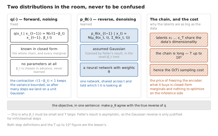
Figure 3. Two distributions in the room, never to be confused.

Exercises

Try these before reading on; they check the conceptual core of this lesson. Solutions are in the collapsible blocks.

1. Why freeze the encoder? A standard VAE learns its encoder $q_\phi(z\mid x)$. A diffusion model instead fixes the “encoder” to the noising chain $q(x_{1:T}\mid x_0)$. State two concrete consequences of this choice — one that makes diffusion easier than a hierarchical VAE, and one that is the price paid.

Easier: because $q$ has no parameters $\phi$, there is nothing to optimize on the inference side — we avoid the encoder-posterior optimization that destabilizes deep hierarchical VAEs, and (Lesson 2) the forward marginals $q(x_t\mid x_0)$ are available in closed form, so we can jump to any noise level in one operation. Price: the latents $x_{1:T}$ share the full dimensionality of the data and the chain is long ($T$ up to $10^3$), giving the $O(T)$ sampling cost.

2. Reading the landscape table. Which generative family offers both exact log-likelihood and single-pass sampling, and what does it pay for that? What does diffusion give up by comparison, and what does it buy?

Normalizing flows give exact $\log p_\theta$ and one-pass sampling, paying with architectural invertibility constraints and expensive Jacobian log-determinants. Diffusion gives up exact likelihood (only an ELBO) and fast sampling ($O(T)$ passes), but buys a stable, well-posed regression objective (no min–max game) and high sample quality.

3. The intractable marginal. Write the integral that defines $p_\theta(x_0)$ from the reverse joint $p_\theta(x_{0:T})$, and say in one sentence why it is intractable (hence why we need the bound of Lesson 4).

$$ p_\theta(x_0)=\int p_\theta(x_{0:T})\,dx_{1:T}=\int p(x_T)\prod_{t=1}^{T}p_\theta(x_{t-1}\mid x_t)\,dx_{1:T}. $$

It is a high-dimensional integral over every latent trajectory $x_{1:T}$ with no closed form, so $\log p_\theta(x_0)$ cannot be evaluated directly — motivating the variational lower bound.

Conclusion

A diffusion model rests on a deliberate asymmetry: a fixed, parameter-free forward process that drowns data in noise, and a learned reverse process that removes noise one gentle step at a time. Formally it is a hierarchical latent-variable model — a VAE whose encoder is frozen to the noising chain — trained by the same ELBO machinery but with a stable regression-like objective. We carry forward two characters, the fixed $q$ and the learned $p_\theta$, and one mission: make the learned reverse match the true reverse of the noising process. In Lesson 2 we make the forward process concrete and uncover the single most useful property in all of diffusion modeling: the closed-form jump to any noise level $t$.

That is the altitude view. The wish we opened with — to run destruction backwards and have something new fall out — is no longer a daydream but a plan with a shape. Lesson 2 begins where it must: by understanding the destruction itself, in enough detail that we will later dare to reverse it.

References

1. Sohl-Dickstein, J., Weiss, E., Maheswaranathan, N., & Ganguli, S. (2015). Deep Unsupervised Learning using Nonequilibrium Thermodynamics. ICML.
2. Ho, J., Jain, A., & Abbeel, P. (2020). Denoising Diffusion Probabilistic Models (DDPM). NeurIPS.
3. Kingma, D. P., & Welling, M. (2014). Auto-Encoding Variational Bayes (VAE). ICLR.
4. Goodfellow, I., Pouget-Abadie, J., Mirza, M., Xu, B., Warde-Farley, D., Ozair, S., Courville, A., & Bengio, Y. (2014). Generative Adversarial Nets. NeurIPS.
5. Rezende, D. J., & Mohamed, S. (2015). Variational Inference with Normalizing Flows. ICML.
6. Yang, L., Zhang, Z., Song, Y., et al. (2023). Diffusion Models: A Comprehensive Survey of Methods and Applications. ACM Computing Surveys.

---

Course Index · Next: Lesson 2 — The Forward Process → · Appendix A: Acronyms · Appendix B: Formulas

---

The figures in this lesson follow the shared figure key , which explains what every shape, line style and colour means.