Lesson 2 — The Forward Process: Destroying Structure with Noise

Recap of Lesson 1. A diffusion model is built on an asymmetry: a fixed forward process $q$ that gradually turns data $x_0$ into pure noise $x_T$, and a learned reverse process $p_\theta$ that denoises step by step. Generation = running the learned reverse from noise. We met the single forward step $q(x_t\mid x_{t-1}) = \mathcal{N}(x_t; \sqrt{1-\beta_t}\,x_{t-1}, \beta_t I)$ and the assumed-Gaussian reverse step. Now we make the forward side completely rigorous.

Suppose you needed to know what a photograph looks like after seven hundred specks of dust have settled on it. The honest method is to drop them one at a time and watch — seven hundred patient steps before you can even begin to work. It is precisely the kind of bookkeeping that makes a method too expensive to love. This lesson finds the shortcut: a single formula that hands you the seven-hundredth state directly, with no waiting in between. Almost everything cheap and practical about training a diffusion model traces back to this one act of teleportation.

Overview

Pouring sand one handful at a time has a cost: to know the photo after $700$ handfuls you would seemingly simulate all $700$ pourings in order, making every gradient step a long sequential simulation. The gift of the Gaussian forward process is that you can teleport: a closed-form expression gives the distribution of $x_t$ directly from $x_0$, for any $t$, with no intermediate simulation. Pick a random noise level, jump there, train. This single fact is what makes diffusion training cheap.

The forward process, formally

The forward (diffusion) process is a Markov chain that injects Gaussian noise according to a variance schedule $\beta_1,\dots,\beta_T$:

Markov means each step depends only on the immediately previous state. There are no learnable parameters; $\beta_t$ is fixed in advance. By the Gaussian reparameterization, drawing $x_t$ is the deterministic update

The factor $\sqrt{1-\beta_t}\lt 1$ contracts the signal; the additive $\sqrt{\beta_t}\,\epsilon$ injects fresh noise. This balance keeps the total variance stable — formally, this is a variance-preserving (VP) process: if $\mathrm{Var}(x_{t-1})=I$ then $\mathrm{Var}(x_t)=(1-\beta_t)I+\beta_t I=I$.

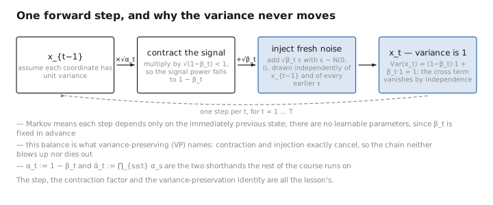
Figure 1. One forward step, and why the variance never moves.

The key trick: jumping to any $t$ in closed form

Here is where the forward process stops being a chore and becomes a gift.

Introduce two shorthand quantities:

Claim.

Lemma: sum of independent Gaussians

We will repeatedly use the following. If $u\sim\mathcal N(0,a^2 I)$ and $v\sim\mathcal N(0,b^2 I)$ are independent, then $u+v\sim\mathcal N(0,(a^2+b^2)I)$. This holds because the sum of independent Gaussians is Gaussian (closure under convolution), the mean is $0+0=0$ by linearity, and for independent variables variances add: $\mathrm{Var}(u+v)=\mathrm{Var}(u)+\mathrm{Var}(v)=(a^2+b^2)I$, the cross term $2\,\mathrm{Cov}(u,v)$ vanishing by independence. Crucially, in the chain each $\epsilon_{t-1}$ is drawn fresh and independently of all $\epsilon_{\lt t-1}$ and of $x_0$, so the independence hypothesis is satisfied at every collapse below.

Derivation by induction

We prove $q(x_t\mid x_0)=\mathcal N(\sqrt{\bar\alpha_t}\,x_0,(1-\bar\alpha_t)I)$ by induction on $t$.

Base case ($t=1$). From the single step, $x_1=\sqrt{\alpha_1}\,x_0+\sqrt{1-\alpha_1}\,\epsilon_0$. Since $\bar\alpha_1=\alpha_1$, this is exactly $x_1=\sqrt{\bar\alpha_1}\,x_0+\sqrt{1-\bar\alpha_1}\,\epsilon_0$, i.e. $q(x_1\mid x_0)=\mathcal N(\sqrt{\bar\alpha_1}\,x_0,(1-\bar\alpha_1)I)$. ✓

Inductive step. Assume $x_{t-1}=\sqrt{\bar\alpha_{t-1}}\,x_0+\sqrt{1-\bar\alpha_{t-1}}\,\bar\epsilon_{t-1}$ with $\bar\epsilon_{t-1}\sim\mathcal N(0,I)$ independent of the next-drawn $\epsilon_{t-1}$. Apply one more forward step:

The deterministic part is $\sqrt{\alpha_t\bar\alpha_{t-1}}\,x_0=\sqrt{\bar\alpha_t}\,x_0$, since $\alpha_t\bar\alpha_{t-1}=\bar\alpha_t$. The two noise terms,

are independent zero-mean Gaussians, so by the Lemma their sum is $\mathcal N(0,c\,I)$ with

Hence $x_t=\sqrt{\bar\alpha_t}\,x_0+\sqrt{1-\bar\alpha_t}\,\bar\epsilon_t$ with $\bar\epsilon_t\sim\mathcal N(0,I)$, i.e. $q(x_t\mid x_0)=\mathcal N(\sqrt{\bar\alpha_t}\,x_0,(1-\bar\alpha_t)I)$. This is the claim at level $t$, completing the induction. $\blacksquare$

Remark (one telescoping line). Unrolling the recursion to $x_0$ directly, the signal coefficient telescopes to $\prod_{s=1}^t\sqrt{\alpha_s}=\sqrt{\bar\alpha_t}$, and the accumulated independent noise contributes variance $\sum_{s=1}^t \big(\prod_{r\gt s}\alpha_r\big)(1-\alpha_s)$, a telescoping sum equal to $1-\bar\alpha_t$. The induction above is just the bookkeeping for this collapse.

Why this is the most important equation in the course

• Cheap training. A noisy sample at level $t$ costs one operation: sample $\epsilon$, compute $\sqrt{\bar\alpha_t}\,x_0+\sqrt{1-\bar\alpha_t}\,\epsilon$. No sequential simulation.
• Signal–noise interpretation. $\sqrt{\bar\alpha_t}$ is the surviving signal, $\sqrt{1-\bar\alpha_t}$ the accumulated noise; their squares sum to $1$, so $x_t$ keeps unit variance.
• The label is the noise. Once $x_t=\sqrt{\bar\alpha_t}\,x_0+\sqrt{1-\bar\alpha_t}\,\epsilon$, the specific $\epsilon$ drawn is the ground truth the network will predict — the seed of the Lesson 5 loss.

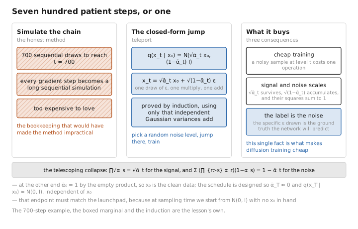
Figure 2. Seven hundred patient steps, or one.

The noise schedule and signal-to-noise ratio

We have been treating the $\beta_t$’s as simply given; it is time to ask who chooses them, and how that choice shapes the entire descent from photograph to static.

Define the signal-to-noise ratio at step $t$ as

$\mathrm{SNR}(t)$ decreases monotonically from $\mathrm{SNR}(0)=\infty$ (clean data) toward $\mathrm{SNR}(T)\approx 0$ (pure noise). The schedule controls how fast $\log\mathrm{SNR}$ descends, and recent work shows the objective and sampling can be parameterized entirely through $\log\mathrm{SNR}$ rather than $\beta_t$ (Kingma et al., 2021).

Linear schedule (DDPM). $\beta_t$ increases linearly, e.g. from $\beta_1=10^{-4}$ to $\beta_T=0.02$ over $T=1000$. Simple, but $\log\mathrm{SNR}$ collapses quickly near the end, so the last steps carry little information.

Cosine schedule (Nichol & Dhariwal). Defines $\bar\alpha_t$ directly to keep more information at high $t$:

for a small offset $s$ (e.g. $0.008$), with $\beta_t=1-\bar\alpha_t/\bar\alpha_{t-1}$ clipped below $\sim0.999$ for stability. This yields a gentler, near-linear $\log\mathrm{SNR}$ decay and improves both likelihood and sample quality.

Remark (continuous-time / VP-SDE). Letting $T\to\infty$ and $\beta_t\to\beta(t)\,dt$, the forward chain becomes the variance-preserving SDE $dx = -\tfrac12\beta(t)\,x\,dt + \sqrt{\beta(t)}\,dw$ (Song et al., 2021). Then $\bar\alpha_t=\exp\!\big(-\!\int_0^t\beta(s)\,ds\big)$, and the discrete VP chain is its Euler–Maruyama discretization. The schedule is just the choice of $\beta(t)$, equivalently the $\log\mathrm{SNR}$ trajectory.

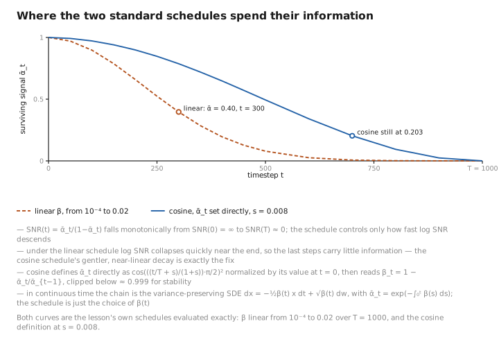
Figure 3. Where the two standard schedules spend their information.

The boundary conditions

As $t\to T$, the schedule is designed so $\bar\alpha_T\approx 0$, giving $q(x_T\mid x_0)\approx\mathcal N(0,I)$ — the data is washed out and the endpoint is (almost) a standard Gaussian, independent of $x_0$. This is essential: at sampling time we start from $\mathcal N(0,I)$ without any $x_0$, and that launchpad must match $q(x_T)$. At the other end, $\bar\alpha_0=1$ (empty product), so $x_0$ is the clean data.

Code & numerics

A reference implementation of the schedule and the one-shot forward jump. Shapes assume images $x_0$ of shape (B, C, H, W).

import torch

def make_alpha_bar(T=1000, beta_start=1e-4, beta_end=2e-2, device="cpu"):
    # betas: (T,)  -> alphas: (T,)  -> alpha_bar via cumulative product
    betas = torch.linspace(beta_start, beta_end, T, device=device)  # (T,)
    alphas = 1.0 - betas                                            # (T,)
    alpha_bar = torch.cumprod(alphas, dim=0)                        # (T,) = prod_{s<=t} alpha_s
    return betas, alphas, alpha_bar

def forward_jump(x0, t, alpha_bar):
    # x0: (B, C, H, W) ; t: (B,) integer step indices in [0, T)
    # returns x_t and the noise epsilon used as the training label
    ab_t = alpha_bar[t]                       # (B,)
    # reshape for broadcasting against (B, C, H, W)
    sqrt_ab   = ab_t.sqrt().view(-1, 1, 1, 1)         # (B,1,1,1)
    sqrt_1mab = (1.0 - ab_t).clamp(min=0).sqrt().view(-1, 1, 1, 1)
    eps = torch.randn_like(x0)                # (B, C, H, W) ~ N(0, I)
    x_t = sqrt_ab * x0 + sqrt_1mab * eps      # closed-form q(x_t | x_0)
    return x_t, eps

Numerical notes.

• Use torch.cumprod once and cache alpha_bar; never recompute the product per batch.
• 1 - alpha_bar can underflow toward $0$ at small $t$ and toward machine-epsilon error near $t=0$; .clamp(min=0) guards the sqrt against tiny negative values from float rounding. Near $t=T$, $\bar\alpha_T$ is extremely small but should stay $\gt 0$ — if a schedule drives it to exactly $0$, $\mathrm{SNR}$ and any $1/\sqrt{\bar\alpha_t}$ term (used in $x_0$-prediction reparameterizations) diverge.
• Prefer float32 (or float64 for the cumprod) when $T$ is large: a long product of numbers $\lt 1$ accumulates rounding; computing $\log\bar\alpha_t=\sum_s\log\alpha_s$ via torch.cumsum(torch.log(alphas)) is more stable, then exponentiate.
• Index alpha_bar[t] with an integer tensor of shape (B,), then .view(-1,1,1,1) to broadcast cleanly across channels and spatial dims.

Exercises

1. Variance preservation. Assume each coordinate of $x_{t-1}$ has unit variance and is independent of the fresh noise $\epsilon_{t-1}\sim\mathcal N(0,I)$. Show the single forward step $x_t=\sqrt{1-\beta_t}\,x_{t-1}+\sqrt{\beta_t}\,\epsilon_{t-1}$ leaves the variance equal to $1$.

the cross term $2\sqrt{(1-\beta_t)\beta_t}\,\mathrm{Cov}(x_{t-1},\epsilon_{t-1})$ vanishing by independence. Hence “variance-preserving.”

2. Moments and SNR. Using the closed form $x_t=\sqrt{\bar\alpha_t}\,x_0+\sqrt{1-\bar\alpha_t}\,\epsilon$, compute $\mathbb E[x_t\mid x_0]$ and $\mathrm{Var}(x_t\mid x_0)$, and confirm that the ratio of signal power to noise power is $\mathrm{SNR}(t)=\bar\alpha_t/(1-\bar\alpha_t)$ (take $\mathrm{Var}(x_0)\approx1$).

$\mathbb E[x_t\mid x_0]=\sqrt{\bar\alpha_t}\,x_0$ (since $\mathbb E[\epsilon]=0$) and $\mathrm{Var}(x_t\mid x_0)=(1-\bar\alpha_t)I$. The deterministic “signal” part carries power $\bar\alpha_t\,\mathrm{Var}(x_0)\approx\bar\alpha_t$; the noise part carries power $1-\bar\alpha_t$. Their ratio is $\bar\alpha_t/(1-\bar\alpha_t)=\mathrm{SNR}(t)$.

3. A two-step jump from scratch. Without invoking the general closed form, compose two forward steps to express $x_t$ in terms of $x_{t-2}$, and show $x_t=\sqrt{\alpha_t\alpha_{t-1}}\,x_{t-2}+\sqrt{1-\alpha_t\alpha_{t-1}}\,\bar\epsilon$ with $\bar\epsilon\sim\mathcal N(0,I)$. (This is the induction’s inductive step in miniature.)

Write $x_t=\sqrt{\alpha_t}\,x_{t-1}+\sqrt{1-\alpha_t}\,\epsilon_{t-1}$ and $x_{t-1}=\sqrt{\alpha_{t-1}}\,x_{t-2}+\sqrt{1-\alpha_{t-1}}\,\epsilon_{t-2}$. Substituting,

By the variance-addition lemma the noise term is $\mathcal N(0,c\,I)$ with $c=\alpha_t(1-\alpha_{t-1})+(1-\alpha_t)=1-\alpha_t\alpha_{t-1}$. Hence $x_t=\sqrt{\alpha_t\alpha_{t-1}}\,x_{t-2}+\sqrt{1-\alpha_t\alpha_{t-1}}\,\bar\epsilon$ — the $\bar\alpha$ pattern with a two-factor product.

4. Numerical stability of $\bar\alpha_t$. Explain why computing $\log\bar\alpha_t=\sum_{s\le t}\log\alpha_s$ via a cumulative sum of logs is more stable for $T\sim1000$ than forming $\bar\alpha_t=\prod_{s\le t}\alpha_s$ and then taking a log.

$\bar\alpha_t$ is a product of $\sim\!1000$ factors each in $(0,1)$, so it shrinks toward (and near $t=T$ very close to) zero — the running product underflows and accumulates multiplicative rounding error, and $\log$ of a near-zero value is ill-conditioned. Summing logs keeps every summand $O(1)$, avoids underflow entirely, and accumulates only additive round-off; exponentiating at the end recovers $\bar\alpha_t$ accurately.

Conclusion

The forward process is a fixed, variance-preserving Gaussian Markov chain that contracts the signal and injects noise step by step. Its defining gift is the closed-form jump $x_t=\sqrt{\bar\alpha_t}\,x_0+\sqrt{1-\bar\alpha_t}\,\epsilon$ — which we proved rigorously by induction using the independence and variance-addition of Gaussians — letting us sample any noise level instantly and exposing $\epsilon$ as the natural training target. We made the schedule precise (linear vs. cosine), defined $\mathrm{SNR}=\bar\alpha_t/(1-\bar\alpha_t)$ and its continuous-time VP-SDE limit, and saw why $x_T$ lands on $\mathcal N(0,I)$. In Lesson 3 we turn around: what does the reverse step look like, why is it also Gaussian, and what exactly must the network compute?

The teleport is in hand: we can now stand at any noise level instantly, the seven-hundredth speck reached in a single stroke. That settles the easy direction. In Lesson 3 we turn around to face the hard one and ask what it would take to step back toward the light — and why, surprisingly, the answer is again a Gaussian.

References

1. Ho, J., Jain, A., & Abbeel, P. (2020). Denoising Diffusion Probabilistic Models (DDPM). NeurIPS.
2. Nichol, A., & Dhariwal, P. (2021). Improved Denoising Diffusion Probabilistic Models (cosine schedule). ICML.
3. Kingma, D. P., Salimans, T., Poole, B., & Ho, J. (2021). Variational Diffusion Models (SNR / log-SNR view). NeurIPS.
4. Song, Y., Sohl-Dickstein, J., Kingma, D. P., Kumar, A., Ermon, S., & Poole, B. (2021). Score-Based Generative Modeling through Stochastic Differential Equations (VP-SDE). ICLR.

← Previous: Lesson 1 — The Big Picture · Course Index · Next: Lesson 3 — The Reverse Process → · Appendix A: Acronyms · Appendix B: Formulas

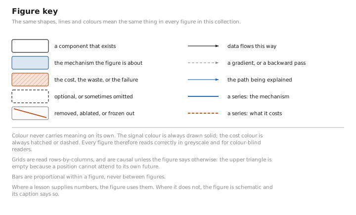
The figures in this lesson follow the shared figure key , which explains what every shape, line style and colour means.