Lesson 3 — The Reverse Process: Learning to Denoise

Recap of Lesson 2. The forward process is a fixed Gaussian Markov chain, $q(x_t\mid x_{t-1}) = \mathcal{N}(x_t; \sqrt{1-\beta_t}\,x_{t-1}, \beta_t I)$. With $\alpha_t = 1-\beta_t$ and $\bar\alpha_t=\prod_{s\le t}\alpha_s$, we proved the closed-form jump $x_t = \sqrt{\bar\alpha_t}\,x_0 + \sqrt{1-\bar\alpha_t}\,\epsilon$, so any noise level is one operation away, and $x_T\approx\mathcal N(0,I)$. The noise $\epsilon$ is the natural training target. Now we build the reverse direction.

Hand a conservator a smudged painting and ask which stroke to undo first, and the honest answer is unsettling: it depends on what the painting was, and that is exactly what you cannot know. But change the rules of the game. Suppose that, while you are still in training, someone quietly lets you see the original. Now the question has a clean, exact answer — you can name the step back to the last coefficient. This lesson is built on that act of permitted cheating: we cannot invert noise out in the open, but conditioned on the clean image we can, and from there we teach a network to manage without the glimpse.

Overview

To generate, we must invert the chain: start at pure noise $x_T\sim\mathcal N(0,I)$ and, step by step, sample a slightly-cleaner $x_{t-1}$ from $x_t$. The honest object is the true reverse conditional $q(x_{t-1}\mid x_t)$. It is intractable: Bayes’ rule writes it as $q(x_{t-1}\mid x_t)=q(x_t\mid x_{t-1})\,q(x_{t-1})/q(x_t)$, and the marginal $q(x_t)=\int q(x_t\mid x_0)\,q(x_0)\,dx_0$ depends on the unknown data distribution $q(x_0)$. We therefore (a) approximate the reverse step with a parametric Gaussian $p_\theta$, justified asymptotically by a result of Feller, and (b) construct a tractable surrogate target by additionally conditioning on $x_0$ — available during training.

Why the reverse step is (approximately) Gaussian

The functional-form license for modeling each reverse step as a Gaussian is a small-noise (diffusion-limit) statement.

Feller’s result. For a diffusion process with continuous sample paths governed by infinitesimal Gaussian transitions (locally Brownian dynamics with bounded drift and diffusion coefficients), the time-reversed process is itself a diffusion with Gaussian infinitesimal transitions (Feller 1949; made precise for the reverse-time SDE by Anderson 1982, which we revisit in Lesson 9). Concretely, as the step size $\beta_t\to 0$, the transition $q(x_{t-1}\mid x_t)$ converges to a Gaussian whose mean is $x_t$ plus an $O(\beta_t)$ score-driven correction and whose covariance is $\beta_t I + o(\beta_t)$.

Rigor remark. This is an asymptotic, small-step statement, not an exact identity for finite $\beta_t$. For finite step size the true $q(x_{t-1}\mid x_t)$ is a Gaussian mixture (an $x_0$-average of the tractable posteriors derived below), hence generally non-Gaussian and multimodal. The Gaussian parametrization of $p_\theta$ incurs an $O(\beta_t^2)$ per-step bias; the bias accumulates over $T$ steps but vanishes in the joint limit $T\to\infty$, $\max_t\beta_t\to0$ with $\bar\alpha_T$ held fixed. This is the formal reason the schedule uses many small steps: it is what makes the Gaussian reverse model consistent, not merely a quality heuristic.

We therefore posit

and define the full reverse (generative) model as the Markov chain

A single network, shared across $t$ and conditioned on $t$ (via a time embedding), emits the mean $\mu_\theta(x_t,t)$ and optionally the covariance.

The tractable posterior

The honest object is out of reach, so we strike a bargain: we will solve a nearby problem we can write down, and arrange for the network to inherit its answer.

While $q(x_{t-1}\mid x_t)$ is intractable, the forward posterior $q(x_{t-1}\mid x_t,x_0)$ — conditioning additionally on the clean image — is exactly Gaussian and available in closed form. During training we hold $x_0$, so we use $q(x_{t-1}\mid x_t,x_0)$ as the ground-truth regression target for $p_\theta(x_{t-1}\mid x_t)$.

By Bayes’ rule, and the forward Markov property $q(x_t\mid x_{t-1},x_0)=q(x_t\mid x_{t-1})$:

Every factor is a known Gaussian (Lesson 2). A product/ratio of Gaussian densities in $x_{t-1}$ is Gaussian, so

Full derivation of $\tilde\beta_t$ and $\tilde\mu_t$

We complete the square. The three relevant densities are

and $q(x_t\mid x_0)$, which does not depend on $x_{t-1}$ and is absorbed into the normalizer. Working component-wise (the covariances are isotropic, so each coordinate decouples), the log of the unnormalized posterior, keeping only $x_{t-1}$-dependent terms, is

Expand both squares and group powers of $x_{t-1}$:

$$ = -\frac{1}{2}\left[\left(\frac{\alpha_t}{\beta_t}+\frac{1}{1-\bar\alpha_{t-1}}\right)x_{t-1}^2

• 2\left(\frac{\sqrt{\alpha_t}}{\beta_t},x_t + \frac{\sqrt{\bar\alpha_{t-1}}}{1-\bar\alpha_{t-1}},x_0\right)x_{t-1}\right]+\text{const}. $$

Matching to the canonical Gaussian exponent $-\tfrac{1}{2}\big(x_{t-1}^2/\tilde\beta_t - 2\,\tilde\mu_t\, x_{t-1}/\tilde\beta_t\big)$ identifies the precision (coefficient of $x_{t-1}^2$):

Verifying $1-\bar\alpha_t = \alpha_t(1-\bar\alpha_{t-1})+\beta_t$. Expand the right side using $\beta_t=1-\alpha_t$ and $\bar\alpha_t=\alpha_t\bar\alpha_{t-1}$:

Hence the numerator is $1-\bar\alpha_t$, and inverting the precision gives

The mean equals (linear coefficient) $\times\,\tilde\beta_t$:

Substitute $\tilde\beta_t=\dfrac{(1-\bar\alpha_{t-1})\beta_t}{1-\bar\alpha_t}$ and simplify each term. For the $x_t$ term, $\dfrac{(1-\bar\alpha_{t-1})\beta_t}{1-\bar\alpha_t}\cdot\dfrac{\sqrt{\alpha_t}}{\beta_t}=\dfrac{\sqrt{\alpha_t}(1-\bar\alpha_{t-1})}{1-\bar\alpha_t}$. For the $x_0$ term, $\dfrac{(1-\bar\alpha_{t-1})\beta_t}{1-\bar\alpha_t}\cdot\dfrac{\sqrt{\bar\alpha_{t-1}}}{1-\bar\alpha_{t-1}}=\dfrac{\sqrt{\bar\alpha_{t-1}}\,\beta_t}{1-\bar\alpha_t}$. Therefore

The two coefficients sum to one only in the noiseless limit; in general the posterior mean is an affine blend of $x_0$ and $x_t$ with schedule-determined weights, plus the variance $\tilde\beta_t\lt \beta_t$ (knowing $x_0$ sharpens the step).

Rigor remark. $\tilde\beta_t$ and $\tilde\mu_t$ depend only on the schedule and on $(x_t,x_0)$, not on $\theta$. They are exact for every finite $\beta_t$; the Gaussian family of the posterior is exact here precisely because we conditioned on $x_0$ (the marginalized version is the mixture noted earlier). At $t=1$, $\bar\alpha_0:=1$, so $\tilde\beta_1=0$ and the posterior is a point mass — handled by the discrete decoder $L_0$ in Lesson 4.

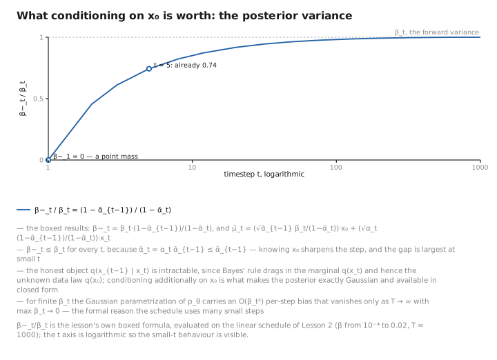
Figure 1. What conditioning on x₀ is worth: the posterior variance.

Rewriting the target in terms of noise

The closed-form jump is invertible:

Substitute this into $\tilde\mu_t$ and carry the algebra through. Insert $x_0$ into the boxed mean:

$$ \tilde\mu_t = \frac{\sqrt{\bar\alpha_{t-1}},\beta_t}{1-\bar\alpha_t}\cdot\frac{1}{\sqrt{\bar\alpha_t}}\big(x_t-\sqrt{1-\bar\alpha_t},\epsilon\big)

• \frac{\sqrt{\alpha_t},(1-\bar\alpha_{t-1})}{1-\bar\alpha_t},x_t. $$

Use $\bar\alpha_t=\alpha_t\bar\alpha_{t-1}$, so $\dfrac{\sqrt{\bar\alpha_{t-1}}}{\sqrt{\bar\alpha_t}}=\dfrac{1}{\sqrt{\alpha_t}}$. The first prefactor becomes $\dfrac{\beta_t}{(1-\bar\alpha_t)\sqrt{\alpha_t}}$. Collect the coefficient of $x_t$:

where the bracket collapsed via the identity $\beta_t+\alpha_t(1-\bar\alpha_{t-1})=1-\bar\alpha_t$ proved above. The coefficient of $\epsilon$ is

Therefore

The optimal reverse mean depends on $x_t$ (available at inference) and on the noise $\epsilon$ that produced it (unknown at inference). If a network predicts that noise, $\epsilon_\theta(x_t,t)\approx\epsilon$, it recovers the ideal denoising mean by substituting $\epsilon_\theta$ in the box. This is why DDPM trains a noise predictor (Lesson 5).

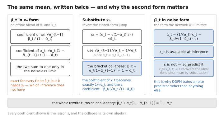
Figure 2. The same mean, written twice — and why the second form matters.

Four equivalent parameterizations

The same reverse step can be carried by any of four different couriers; which one you hire turns out to matter far more for the training than for the truth.

The reverse mean can be carried by any of four equivalent targets, related by invertible linear maps (at fixed $x_t,t$). Let $a_t=\sqrt{\bar\alpha_t}$, $b_t=\sqrt{1-\bar\alpha_t}$, so $x_t=a_t x_0 + b_t\epsilon$.

1. $\mu$-prediction. The network outputs $\mu_\theta(x_t,t)$ directly. Most general but empirically harder to optimize; couples poorly across noise levels.
2. $x_0$-prediction. Output $\hat x_0(x_t,t)$, then set $\mu_\theta=\tilde\mu_t(x_t,\hat x_0)$. Map to noise: $\hat\epsilon=(x_t-a_t\hat x_0)/b_t$. Intuitive, but high-variance loss at large $t$ (small $a_t$).
3. $\epsilon$-prediction (DDPM standard). Output $\epsilon_\theta(x_t,t)$, set $\mu_\theta=\frac{1}{\sqrt{\alpha_t}}\big(x_t-\frac{\beta_t}{\sqrt{1-\bar\alpha_t}}\epsilon_\theta\big)$. Map to $x_0$: $\hat x_0=(x_t-b_t\epsilon_\theta)/a_t$. Cleanest loss (Lesson 5).
4. $v$-prediction (Salimans & Ho 2022). Target $v\equiv a_t\epsilon - b_t x_0$. Inverse maps: $x_0=a_t x_t - b_t v$, $\epsilon=b_t x_t + a_t v$. The map $(x_0,\epsilon)\mapsto(x_t,v)$ is the rotation $\left(\begin{smallmatrix}a_t & b_t\\ -b_t & a_t\end{smallmatrix}\right)$ (since $a_t^2+b_t^2=1$). Behaves well across all SNR, especially near $t=T$ and in distillation.

Rigor remark. All four are exactly equivalent for the optimal predictor and differ only in the loss geometry / implicit per-$t$ weighting they induce; they are not equivalent under a fixed network and finite data. Choosing a parameterization is choosing a reweighting of the per-step objective (Lesson 5).

# Schedule precompute (float64 for stability) and posterior coefficients.
import numpy as np
betas = np.linspace(1e-4, 2e-2, 1000, dtype=np.float64)   # (T,)
alphas = 1.0 - betas
abar = np.cumprod(alphas)                                  # bar_alpha_t, (T,)
abar_prev = np.concatenate([[1.0], abar[:-1]])             # bar_alpha_{t-1}
post_var = betas * (1.0 - abar_prev) / (1.0 - abar)        # tilde_beta_t
# tilde_mu coefficients (eq. for tilde_mu_t(x_t, x_0)):
coef_x0 = np.sqrt(abar_prev) * betas / (1.0 - abar)
coef_xt = np.sqrt(alphas) * (1.0 - abar_prev) / (1.0 - abar)
# Posterior log-variance is clipped at t=1 since tilde_beta_1 = 0:
post_logvar = np.log(np.maximum(post_var, 1e-20))

Numerical note. Compute $\bar\alpha_t$ in float64 and clip $\tilde\beta_t$ before taking logs ($\tilde\beta_1=0$). Prefer $\log(1-\bar\alpha_t)$ via log1p(-abar) when $\bar\alpha_t$ is close to 1 (small $t$) to avoid catastrophic cancellation.

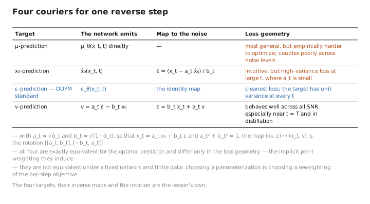
Figure 3. Four couriers for one reverse step.

Exercises

1. Complete the square yourself. From the two relevant log-densities, read off the coefficient of $x_{t-1}^2$ and show the posterior precision is $1/\tilde\beta_t=\alpha_t/\beta_t+1/(1-\bar\alpha_{t-1})$, then invert to recover $\tilde\beta_t=\frac{1-\bar\alpha_{t-1}}{1-\bar\alpha_t}\beta_t$.

The term $-\frac{(x_t-\sqrt{\alpha_t}x_{t-1})^2}{2\beta_t}$ contributes $\frac{\alpha_t}{\beta_t}$ to the coefficient of $x_{t-1}^2$; the term $-\frac{(x_{t-1}-\sqrt{\bar\alpha_{t-1}}x_0)^2}{2(1-\bar\alpha_{t-1})}$ contributes $\frac{1}{1-\bar\alpha_{t-1}}$. Their sum is the precision $1/\tilde\beta_t$. Over the common denominator $\beta_t(1-\bar\alpha_{t-1})$ the numerator is $\alpha_t(1-\bar\alpha_{t-1})+\beta_t=1-\bar\alpha_t$ (the identity proved in the text), so $1/\tilde\beta_t=\frac{1-\bar\alpha_t}{\beta_t(1-\bar\alpha_{t-1})}$, giving $\tilde\beta_t=\frac{1-\bar\alpha_{t-1}}{1-\bar\alpha_t}\beta_t$.

2. Posterior variance ordering. Show $\tilde\beta_t\le\beta_t$ for all $t$, and identify where the ratio approaches $1$ and where the gap is largest.

$\dfrac{\tilde\beta_t}{\beta_t}=\dfrac{1-\bar\alpha_{t-1}}{1-\bar\alpha_t}$. Since $\bar\alpha_t=\alpha_t\bar\alpha_{t-1}\le\bar\alpha_{t-1}$ (because $\alpha_t\le1$), we have $1-\bar\alpha_t\ge1-\bar\alpha_{t-1}$, so the ratio is $\le1$: $\tilde\beta_t\le\beta_t$. As $t\to T$ both $\bar\alpha$’s $\to0$ and the ratio $\to1$. The gap is largest at small $t$; at $t=1$, $\bar\alpha_0:=1$ gives $\tilde\beta_1=0$ (knowing $x_0$ pins $x_0$ exactly — a point mass).

3. From $x_0$-form to noise-form. Substitute $x_0=\frac{1}{\sqrt{\bar\alpha_t}}(x_t-\sqrt{1-\bar\alpha_t}\,\epsilon)$ into $\tilde\mu_t(x_t,x_0)=\frac{\sqrt{\bar\alpha_{t-1}}\beta_t}{1-\bar\alpha_t}x_0+\frac{\sqrt{\alpha_t}(1-\bar\alpha_{t-1})}{1-\bar\alpha_t}x_t$ and verify the coefficient of $x_t$ collapses to $1/\sqrt{\alpha_t}$.

Using $\sqrt{\bar\alpha_{t-1}}/\sqrt{\bar\alpha_t}=1/\sqrt{\alpha_t}$, the $x_0$-term contributes $\frac{\beta_t}{(1-\bar\alpha_t)\sqrt{\alpha_t}}x_t$ (plus an $\epsilon$ piece). Adding the existing $x_t$-coefficient:

using $\beta_t+\alpha_t(1-\bar\alpha_{t-1})=1-\bar\alpha_t$. The $\epsilon$-coefficient works out to $-\frac{\beta_t}{\sqrt{\alpha_t}\sqrt{1-\bar\alpha_t}}$, giving the boxed noise-form mean.

4. Converting between targets. Given a network output $\hat\epsilon$ at $(x_t,t)$, and shorthand $a_t=\sqrt{\bar\alpha_t},\,b_t=\sqrt{1-\bar\alpha_t}$, express $\hat x_0$ and the velocity $v$ purely in terms of $\hat\epsilon$ and $x_t$.

From $x_t=a_t x_0+b_t\epsilon$: $\hat x_0=(x_t-b_t\hat\epsilon)/a_t$. For $v=a_t\epsilon-b_t x_0$, substitute $x_0$ and use $a_t^2+b_t^2=1$:

(Equivalently $\epsilon=b_t x_t+a_t v$, the inverse map of Lesson 5.)

Conclusion

The reverse step is Gaussian asymptotically, because the forward steps are infinitesimal (Feller); for finite $\beta_t$ this is an $O(\beta_t^2)$ approximation, which is why $T$ is large. We cannot access the true reverse conditional, but conditioning on $x_0$ yields the exact tractable posterior $q(x_{t-1}\mid x_t,x_0)=\mathcal N(\tilde\mu_t,\tilde\beta_t I)$, derived in full by completing the square. Substituting $x_0=x_0(x_t,\epsilon)$ gave the noise-form mean, showing that predicting $\epsilon$ suffices to recover the ideal denoiser. We catalogued the four parameterizations and the linear maps between them. Lesson 4 derives why matching this posterior is the principled objective via the variational lower bound.

The glimpse of $x_0$ bought us an exact reverse step to imitate, and a clean reason to predict noise. But “imitate this posterior” is still, at this point, an assertion. Lesson 4 supplies the justification — it shows that matching this step is not a convenient hack but the unavoidable consequence of pushing up a bound on the data’s likelihood.

References

• J. Sohl-Dickstein, E. Weiss, N. Maheswaranathan, S. Ganguli. Deep Unsupervised Learning using Nonequilibrium Thermodynamics. ICML 2015.
• J. Ho, A. Jain, P. Abbeel. Denoising Diffusion Probabilistic Models. NeurIPS 2020.
• W. Feller. On the Theory of Stochastic Processes, with Particular Reference to Applications. Proc. Berkeley Symp. on Math. Stat. and Prob., 1949 (Gaussianity of reverse infinitesimal transitions).
• B. D. O. Anderson. Reverse-Time Diffusion Equation Models. Stochastic Processes and their Applications, 1982 (reverse-time SDE; forward pointer to Lesson 9).
• T. Salimans, J. Ho. Progressive Distillation for Fast Sampling of Diffusion Models. ICLR 2022 ($v$-parameterization).

← Previous: Lesson 2 — The Forward Process · Course Index · Next: Lesson 4 — The Variational Lower Bound → · Appendix A: Acronyms · Appendix B: Formulas

The figures in this lesson follow the shared figure key , which explains what every shape, line style and colour means.