Lesson 4 — The Variational Lower Bound (ELBO)
Recap of Lesson 3. Because forward steps are tiny, the reverse step is Gaussian; we model it as $p_\theta(x_{t-1}\mid x_t)=\mathcal N(x_{t-1};\mu_\theta(x_t,t),\Sigma_\theta)$. The true reverse $q(x_{t-1}\mid x_t)$ is intractable, but conditioning on $x_0$ yields a tractable Gaussian posterior $q(x_{t-1}\mid x_t,x_0)=\mathcal N(\tilde\mu_t,\tilde\beta_t I)$ with closed-form $\tilde\mu_t$ and $\tilde\beta_t$. Rewriting $\tilde\mu_t$ in terms of the noise $\epsilon$ showed that predicting $\epsilon$ recovers the ideal denoiser. This lesson explains why matching that posterior is the principled objective.
There is a number we badly want and cannot have: the likelihood the model assigns to real data. It hides behind an integral over every possible trajectory of noise, and that integral will not be computed in this lifetime. The move that rescues the whole enterprise is older than diffusion and quietly audacious — if you cannot measure the thing itself, measure something you can, and prove it never overshoots. This lesson builds that provable stand-in, the ELBO, and then patiently takes it apart until what is left is something a network can actually be trained on.
Overview
We have a target (the tractable posterior) and a model (the Gaussian reverse step), but not yet the loss that ties them together nor a guarantee that minimizing it improves $p_\theta(x_0)$. The answer is the variational lower bound (ELBO), the latent-variable-model machinery behind the VAE (Kingma & Welling 2014), applied to a $T$-step chain. The marginal likelihood $p_\theta(x_0)=\int p_\theta(x_{0:T})\,dx_{1:T}$ is intractable, so we optimize a tractable bound; pushing the bound up raises the likelihood it supports.
Setting up the bound
We minimize $-\log p_\theta(x_0)$. Two routes give the same bound.
Route 1 — Jensen. Introduce the fixed forward process $q(x_{1:T}\mid x_0)$ as the variational distribution. With $\log$ concave,
$$ -\log p_\theta(x_0) = -\log \int q(x_{1:T}\mid x_0)\,\frac{p_\theta(x_{0:T})}{q(x_{1:T}\mid x_0)}\,dx_{1:T} \le \mathbb{E}_{q}\!\left[-\log\frac{p_\theta(x_{0:T})}{q(x_{1:T}\mid x_0)}\right] =: L. $$Route 2 — exact KL-gap identity. Write $p_\theta(x_{0:T})=p_\theta(x_{1:T}\mid x_0)\,p_\theta(x_0)$ inside $L$:
$$ L = \mathbb{E}_q\!\left[-\log\frac{p_\theta(x_{1:T}\mid x_0)\,p_\theta(x_0)}{q(x_{1:T}\mid x_0)}\right] = -\log p_\theta(x_0) + \mathbb{E}_q\!\left[\log\frac{q(x_{1:T}\mid x_0)}{p_\theta(x_{1:T}\mid x_0)}\right], $$where $-\log p_\theta(x_0)$ leaves the expectation as a constant w.r.t. $q$. Hence the exact gap is
$$ \boxed{\ L - \big(-\log p_\theta(x_0)\big) = D_{\mathrm{KL}}\!\big(q(x_{1:T}\mid x_0)\,\|\,p_\theta(x_{1:T}\mid x_0)\big)\ \ge 0.\ } $$KL non-negativity (Gibbs’ inequality) re-derives Route 1 and makes the slack explicit: $L$ is tight iff the forward posterior equals the model’s reverse posterior. Thus $L$ upper-bounds the negative log-likelihood; $-L$ is the ELBO. Minimizing $L$ is the objective.
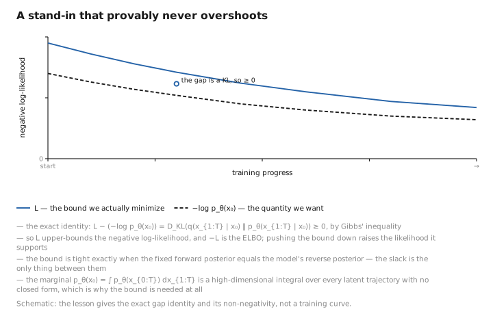
Figure 1. A stand-in that provably never overshoots.
Decomposing the bound into per-step KL terms
A single intractable bound is progress, but not yet something to optimize; we now break it into pieces small enough to recognize one by one.
Expand $L$ with the Markov factorizations of Lessons 2–3:
$$ L = \mathbb{E}_q\!\left[-\log\frac{p(x_T)\prod_{t\ge1}p_\theta(x_{t-1}\mid x_t)}{\prod_{t\ge1}q(x_t\mid x_{t-1})}\right] = \mathbb{E}_q\!\left[-\log p(x_T) - \sum_{t\ge1}\log\frac{p_\theta(x_{t-1}\mid x_t)}{q(x_t\mid x_{t-1})}\right]. $$Split off $t=1$ and, for $t\ge2$, rewrite each forward factor with Bayes (using the Markov property $q(x_t\mid x_{t-1})=q(x_t\mid x_{t-1},x_0)$):
$$ q(x_t\mid x_{t-1}) = \frac{q(x_{t-1}\mid x_t, x_0)\,q(x_t\mid x_0)}{q(x_{t-1}\mid x_0)}. $$Substituting, the $t\ge2$ sum becomes
$$ -\sum_{t\ge2}\log\frac{p_\theta(x_{t-1}\mid x_t)}{q(x_{t-1}\mid x_t,x_0)} \;-\;\sum_{t\ge2}\log\frac{q(x_{t-1}\mid x_0)}{q(x_t\mid x_0)}. $$The telescoping ratio. The second sum telescopes. Writing the summand as $\log q(x_{t-1}\mid x_0)-\log q(x_t\mid x_0)$ for $t=2,\dots,T$:
$$ \sum_{t=2}^{T}\big[\log q(x_{t-1}\mid x_0)-\log q(x_t\mid x_0)\big] = \log q(x_1\mid x_0) - \log q(x_T\mid x_0), $$because every interior term $\log q(x_t\mid x_0)$ (for $2\le t\le T-1$) appears once with each sign and cancels. The surviving $-\big(-\log q(x_1\mid x_0)\big)$ combines with the $t=1$ factor $-\log\frac{p_\theta(x_0\mid x_1)}{q(x_1\mid x_0)}=-\log p_\theta(x_0\mid x_1)+\log q(x_1\mid x_0)$: the two $\log q(x_1\mid x_0)$ pieces cancel, leaving only $-\log p_\theta(x_0\mid x_1)$. The surviving $-\log q(x_T\mid x_0)$ pairs with $-\log p(x_T)$ to form a KL. Taking $\mathbb E_q$ and recognizing $\mathbb E_{q}[-\log\frac{p_\theta}{q}]=D_{\mathrm{KL}}(q\|p_\theta)$ termwise:
$$ \boxed{, L = \underbrace{D_{\mathrm{KL}}!\big(q(x_T\mid x_0),|,p(x_T)\big)}_{L_T}
- \sum_{t=2}^{T}\underbrace{D_{\mathrm{KL}}!\big(q(x_{t-1}\mid x_t,x_0),|,p_\theta(x_{t-1}\mid x_t)\big)}{L{t-1}} \underbrace{-,\log p_\theta(x_0\mid x_1)}_{L_0} ,} $$
A concrete walk-through: telescoping at $T=3$
The general argument above asks you to hold several identities in your head at once. It is worth doing once with all the steps written out on the smallest non-trivial chain, $T=3$. Nothing is hidden here — every term is tracked until it either survives or cancels.
Step 0 — write $L$ explicitly. With $T=3$ the sum $\sum_{t\ge1}$ runs over $t=1,2,3$, so the expression inside $\mathbb E_q$ (call it $A$, so $L=\mathbb E_q[A]$) is
$$ A = -\log p(x_3) \;\underbrace{-\log\frac{p_\theta(x_0\mid x_1)}{q(x_1\mid x_0)}}_{t=1} \;\underbrace{-\log\frac{p_\theta(x_1\mid x_2)}{q(x_2\mid x_1)}}_{t=2} \;\underbrace{-\log\frac{p_\theta(x_2\mid x_3)}{q(x_3\mid x_2)}}_{t=3}. $$Step 1 — leave $t=1$ alone; rewrite the forward factors for $t=2,3$ with Bayes. Using $q(x_t\mid x_{t-1})=\dfrac{q(x_{t-1}\mid x_t,x_0)\,q(x_t\mid x_0)}{q(x_{t-1}\mid x_0)}$:
$$ \log q(x_2\mid x_1)=\log q(x_1\mid x_2,x_0)+\log q(x_2\mid x_0)-\log q(x_1\mid x_0), $$$$ \log q(x_3\mid x_2)=\log q(x_2\mid x_3,x_0)+\log q(x_3\mid x_0)-\log q(x_2\mid x_0). $$Step 2 — substitute and group by type. Expanding $A$ and colour-sorting the pieces:
$$ A = \underbrace{-\log p_\theta(x_0\mid x_1)}_{\to\,L_0} \;\underbrace{-\log\frac{p_\theta(x_1\mid x_2)}{q(x_1\mid x_2,x_0)}}_{\to\,L_1} \;\underbrace{-\log\frac{p_\theta(x_2\mid x_3)}{q(x_2\mid x_3,x_0)}}_{\to\,L_2} \;-\log p(x_3) \;+\;\Big[\,\underbrace{\log q(x_1\mid x_0)}_{\text{from }t=1}+\log q(x_2\mid x_0)-\log q(x_1\mid x_0)+\log q(x_3\mid x_0)-\log q(x_2\mid x_0)\Big]. $$Step 3 — watch the marginal-log terms cancel. Inside the bracket, line up the $\log q(x_t\mid x_0)$ pieces:
| term | sign(s) it appears with | fate |
|---|---|---|
| $\log q(x_1\mid x_0)$ | $+$ (from the $t=1$ factor) and $-$ (from the $t=2$ Bayes step) | cancels |
| $\log q(x_2\mid x_0)$ | $+$ (from $t=2$) and $-$ (from $t=3$) | cancels (an interior term) |
| $\log q(x_3\mid x_0)$ | $+$ (from $t=3$) only | survives |
So the entire bracket collapses to a single survivor, $\log q(x_3\mid x_0)$.
Step 4 — read off the four groups. Pairing the survivor with $-\log p(x_3)$ and taking $\mathbb E_q$ (so each $\mathbb E_q[-\log\frac{p}{q}]$ becomes a $D_{\mathrm{KL}}(q\,\|\,p)$):
$$ L = \underbrace{D_{\mathrm{KL}}\!\big(q(x_3\mid x_0)\,\|\,p(x_3)\big)}_{L_T,\ \ T=3} \;+\;\underbrace{D_{\mathrm{KL}}\!\big(q(x_2\mid x_3,x_0)\,\|\,p_\theta(x_2\mid x_3)\big)}_{L_2} \;+\;\underbrace{D_{\mathrm{KL}}\!\big(q(x_1\mid x_2,x_0)\,\|\,p_\theta(x_1\mid x_2)\big)}_{L_1} \;\underbrace{-\,\log p_\theta(x_0\mid x_1)}_{L_0}. $$This is exactly the boxed formula with $T=3$: one prior term $L_T$, the denoising sum $\sum_{t=2}^{3}L_{t-1}=L_2+L_1$, and the reconstruction term $L_0$. The two cancellations in Step 3 are the whole content of “the telescoping ratio”; for general $T$ the same bookkeeping leaves every interior $\log q(x_t\mid x_0)$ paired off, with only the endpoints $\log q(x_1\mid x_0)$ (absorbed into $L_0$) and $\log q(x_T\mid x_0)$ (forming $L_T$) untouched.
Each piece has a clear role:
- $L_T$ — prior matching. $D_{\mathrm{KL}}(q(x_T\mid x_0)\,\|\,\mathcal N(0,I))$ has no learnable parameters (forward process fixed), so it is a constant in $\theta$, ignorable during optimization, and is small by design ($\bar\alpha_T\approx0$).
- $L_{t-1}$ — denoising matching (the heart). Each compares the model reverse step to the tractable posterior of Lesson 3; the $T-1$ terms carry essentially all learning signal.
- $L_0$ — reconstruction. Decoding $x_1\to x_0$ to discrete data, handled by a separate discretized-likelihood model (Ho et al. 2020).
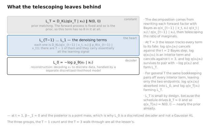
Figure 2. What the telescoping leaves behind.
Evaluating the denoising terms: Gaussian KL
Each surviving piece is a divergence between two Gaussians — and that is a piece of real luck, because there are few quantities in all of statistics we can write down more explicitly.
The decomposition pays off because both arguments of each $L_{t-1}$ are Gaussians. For two $d$-dimensional Gaussians the KL is closed-form. General diagonal case $\mathcal N(\mu_1,\Sigma_1)\,\|\,\mathcal N(\mu_2,\Sigma_2)$:
$$ D_{\mathrm{KL}} = \frac{1}{2}\!\left[\operatorname{tr}(\Sigma_2^{-1}\Sigma_1) + (\mu_2-\mu_1)^\top\Sigma_2^{-1}(\mu_2-\mu_1) - d + \log\frac{\det\Sigma_2}{\det\Sigma_1}\right]. $$Equal covariance $\Sigma_1=\Sigma_2=\Sigma$: the trace term equals $d$, the log-det term vanishes, and only the Mahalanobis mean gap survives:
$$ D_{\mathrm{KL}}\!\big(\mathcal N(\tilde\mu,\Sigma)\,\|\,\mathcal N(\mu_\theta,\Sigma)\big) = \frac{1}{2}\,(\tilde\mu - \mu_\theta)^\top \Sigma^{-1} (\tilde\mu - \mu_\theta). $$Isotropic specialization $\Sigma=\sigma_t^2 I$, so $\Sigma^{-1}=\sigma_t^{-2}I$:
$$ \boxed{\ L_{t-1} = \frac{1}{2\sigma_t^2}\,\big\|\tilde\mu_t(x_t,x_0) - \mu_\theta(x_t,t)\big\|^2 + C.\ } $$DDPM fixes the reverse covariance to a schedule constant, $\Sigma_\theta=\sigma_t^2 I$ with $\sigma_t^2=\beta_t$ or $\sigma_t^2=\tilde\beta_t$ (comparable in practice), which is exactly the equal-covariance condition that drops every term but the mean gap. The grand variational objective has reduced to mean-matching regression weighted by $1/2\sigma_t^2$.
Rigor remark — learned variance and hybrid loss. Fixing $\sigma_t^2$ is a modeling choice. Improved DDPM (Nichol & Dhariwal 2021) learns the reverse variance as a per-coordinate interpolation in log-space, $\Sigma_\theta=\exp\!\big(v\log\beta_t+(1-v)\log\tilde\beta_t\big)$, with $v=v_\theta(x_t,t)\in[0,1]$ keeping the variance bracketed by the two natural bounds $\tilde\beta_t\le\Sigma_\theta\le\beta_t$. With learned $\Sigma_\theta$ the full Gaussian KL (trace and log-det terms) no longer cancels, so $L_{t-1}$ must be evaluated in full. They optimize a hybrid loss $L_{\text{hybrid}}=L_{\text{simple}}+\lambda L_{\text{vlb}}$ (typically $\lambda=10^{-3}$), with a stop-gradient on $\mu_\theta$ inside $L_{\text{vlb}}$ so the simple loss trains the mean and the VLB term trains only the variance. This improves log-likelihood (NLL) markedly with negligible sample-quality cost. The continuous-time VDM treatment (Kingma et al. 2021) recasts the bound as an SNR-weighted integral and shows the weighting, not the parameterization, is what matters.
Numerical note. Evaluate the full Gaussian KL in log-variance space and use closed forms (
tr,log detas sums of diagonal logs) rather than forming $\Sigma^{-1}$. At $t=1$, $\tilde\beta_1=0$, so $L_0$ is the discretized decoder, not a KL; do not feed a degenerate Gaussian into the KL formula.
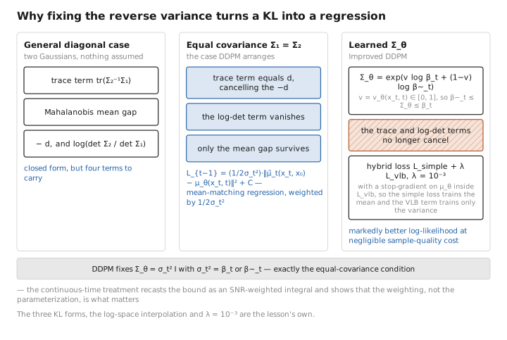
Figure 3. Why fixing the reverse variance turns a KL into a regression.
Exercises
1. The exact KL gap. Starting from $L=\mathbb E_q[-\log\frac{p_\theta(x_{0:T})}{q(x_{1:T}\mid x_0)}]$, use $p_\theta(x_{0:T})=p_\theta(x_{1:T}\mid x_0)\,p_\theta(x_0)$ to show $L=-\log p_\theta(x_0)+D_{\mathrm{KL}}(q(x_{1:T}\mid x_0)\,\|\,p_\theta(x_{1:T}\mid x_0))$, and hence $L\ge-\log p_\theta(x_0)$.
Substituting the factorization,
$$ L=\mathbb E_q\!\left[-\log\frac{p_\theta(x_{1:T}\mid x_0)\,p_\theta(x_0)}{q(x_{1:T}\mid x_0)}\right] =-\log p_\theta(x_0)+\mathbb E_q\!\left[\log\frac{q(x_{1:T}\mid x_0)}{p_\theta(x_{1:T}\mid x_0)}\right], $$because $-\log p_\theta(x_0)$ has no $x_{1:T}$ dependence and leaves the expectation. The remaining expectation is exactly $D_{\mathrm{KL}}(q(x_{1:T}\mid x_0)\,\|\,p_\theta(x_{1:T}\mid x_0))\ge0$ by Gibbs’ inequality, so $L\ge-\log p_\theta(x_0)$.
2. Telescope at $T=2$. Redo the worked walk-through for the minimal chain $T=2$ and show $L=D_{\mathrm{KL}}(q(x_2\mid x_0)\,\|\,p(x_2))+D_{\mathrm{KL}}(q(x_1\mid x_2,x_0)\,\|\,p_\theta(x_1\mid x_2))-\log p_\theta(x_0\mid x_1)$. Which cancellation from the $T=3$ case is now absent?
For $T=2$ the sum runs over $t=1,2$. The $t=1$ factor keeps $+\log q(x_1\mid x_0)$; the $t=2$ Bayes step gives $+\log q(x_1\mid x_2,x_0)+\log q(x_2\mid x_0)-\log q(x_1\mid x_0)$. The two $\log q(x_1\mid x_0)$ pieces cancel; $\log q(x_2\mid x_0)$ pairs with $-\log p(x_2)$ to form $L_T$; $-\log p_\theta(x_1\mid x_2)+\log q(x_1\mid x_2,x_0)$ is $L_1$; and $-\log p_\theta(x_0\mid x_1)$ is $L_0$. There is no interior cancellation (no $\log q(x_2\mid x_0)$-type term appearing with both signs) — $T=2$ is the smallest chain, so only the endpoint cancellation occurs.
3. Equal-covariance KL collapse. Starting from the general diagonal-Gaussian KL, set $\Sigma_1=\Sigma_2=\Sigma$ and show it reduces to $\tfrac12(\mu_2-\mu_1)^\top\Sigma^{-1}(\mu_2-\mu_1)$.
With $\Sigma_1=\Sigma_2=\Sigma$: the trace term $\operatorname{tr}(\Sigma^{-1}\Sigma)=\operatorname{tr}(I)=d$ cancels the $-d$; the log-det term $\log\frac{\det\Sigma}{\det\Sigma}=0$. Only the Mahalanobis mean-gap term $\tfrac12(\mu_2-\mu_1)^\top\Sigma^{-1}(\mu_2-\mu_1)$ survives — which is why fixing the reverse covariance to a schedule constant turns each $L_{t-1}$ into pure mean-matching.
4. Why $L_T$ is free. Explain why $L_T$ carries no learnable parameters, and why it is small by design.
$L_T=D_{\mathrm{KL}}(q(x_T\mid x_0)\,\|\,p(x_T))$ compares the fixed forward marginal $q(x_T\mid x_0)$ (no $\theta$) with the fixed prior $p(x_T)=\mathcal N(0,I)$ (no $\theta$), so it is a constant in $\theta$ — ignorable for optimization. It is small because the schedule drives $\bar\alpha_T\approx0$, making $q(x_T\mid x_0)\approx\mathcal N(0,I)$, i.e. nearly the prior, so the KL $\to0$.
Conclusion
Maximizing the data likelihood is intractable, so we maximize a variational lower bound; the slack is exactly $D_{\mathrm{KL}}(q(x_{1:T}\mid x_0)\,\|\,p_\theta(x_{1:T}\mid x_0))$. Rewriting the forward factors with the $x_0$-conditioned posterior and telescoping the $q(x_t\mid x_0)/q(x_{t-1}\mid x_0)$ ratios decomposes $L$ into a constant prior term $L_T$, a reconstruction term $L_0$, and the heart — a sum of closed-form Gaussian KL denoising terms $L_{t-1}$. With fixed isotropic reverse variance these collapse to $\frac{1}{2\sigma_t^2}\|\tilde\mu_t-\mu_\theta\|^2$: mean-matching regression. Optional learned variance (Improved DDPM) trades the cancellation for better likelihood via a hybrid loss. In Lesson 5 we substitute the noise parameterization, watch the means cancel, and obtain the one-line DDPM training loss.
We set out to measure something unmeasurable and ended up holding a tidy sum of Gaussian KLs — a constant we can ignore, a reconstruction term, and a heart made of mean-matching. Lesson 5 watches that heart collapse, almost magically, into a single line of regression.
References
- J. Ho, A. Jain, P. Abbeel. Denoising Diffusion Probabilistic Models. NeurIPS 2020.
- J. Sohl-Dickstein, E. Weiss, N. Maheswaranathan, S. Ganguli. Deep Unsupervised Learning using Nonequilibrium Thermodynamics. ICML 2015.
- D. P. Kingma, M. Welling. Auto-Encoding Variational Bayes. ICLR 2014 (ELBO / VAE).
- A. Nichol, P. Dhariwal. Improved Denoising Diffusion Probabilistic Models. ICML 2021 (learned variance, hybrid loss).
- D. P. Kingma, T. Salimans, B. Poole, J. Ho. Variational Diffusion Models. NeurIPS 2021 (continuous-time / SNR-weighted bound).
← Previous: Lesson 3 — The Reverse Process · Course Index · Next: Lesson 5 — The Simplified Objective → · Appendix A: Acronyms · Appendix B: Formulas
The figures in this lesson follow the shared figure key , which explains what every shape, line style and colour means.