Lesson 5 — The Simplified Training Objective

Recap of Lesson 4. We maximize a variational lower bound $L = L_T + \sum_{t\ge2}L_{t-1} + L_0$. The prior term $L_T$ is a parameter-free constant; the reconstruction term $L_0$ is minor; the denoising terms $L_{t-1}$ carry the learning. With fixed reverse variance $\sigma_t^2 I$, each reduces to a weighted squared error between the network’s reverse mean $\mu_\theta(x_t,t)$ and the analytic posterior mean $\tilde\mu_t(x_t,x_0)$: $L_{t-1}=\frac{1}{2\sigma_t^2}\|\tilde\mu_t-\mu_\theta\|^2 + C$. Now we collapse this into one clean loss.

By now we have assembled a fair amount of apparatus: a variational bound, a tractable posterior, a KL between Gaussians, a schedule of fiddly coefficients. It would be reasonable to expect the training objective to look like all of that machinery bolted together. Instead, when the right substitution is made, the apparatus folds in on itself and almost everything cancels — leaving a single line you could explain to someone who has never heard the word “posterior”: look at a noisy image, guess the noise. This lesson is the story of that collapse, and of why the messy weight that drops out is worth throwing away.

Overview

Lesson 4 left the objective in mean-matching form: the regression target $\tilde\mu_t(x_t,x_0)$ from Lesson 3 is a schedule-dependent affine blend of $x_0$ and $x_t$. Asking a network to hit that exact blend couples the optimizer’s target to the noise schedule and rescales it across $t$. The remedy is a change of parameterization. Writing $\tilde\mu_t$ in its noise form and giving $\mu_\theta$ the identical functional shape causes the schedule factors to cancel algebraically, leaving a plain $\ell_2$ regression onto the injected noise $\epsilon$. The DDPM observation is that discarding the per-timestep weight $w_t$ that falls out of the ELBO further improves perceptual sample quality. We make the cancellation explicit, derive $w_t$ exactly, locate the resulting loss in the space of SNR-weighted objectives, and lay out the linear correspondence between $\epsilon$-, $x_0$-, and $v$-targets.

Parameterizing the mean through noise

From Lesson 3, the posterior mean in noise form is

We choose to give the network the same shape, but with a predicted noise $\epsilon_\theta(x_t,t)$ in place of the true $\epsilon$:

This is the $\epsilon$-parameterization. The network’s only job is to look at the noisy $x_t$ (and the timestep $t$) and predict the noise vector $\epsilon$ that contaminated it. Note that this is not the only admissible reparameterization — it is a deliberate one, chosen precisely because it cancels the schedule (below) and because it makes the regression target unit-variance for all $t$ (see Lesson 9, score matching).

The cancellation, in full

Watch closely now; this is the trick the whole lesson turns on.

Substitute both means into the denoising term $L_{t-1}=\frac{1}{2\sigma_t^2}\|\tilde\mu_t-\mu_\theta\|^2$. Write $c_t := 1/\sqrt{\alpha_t}$ and $b_t := \beta_t/\sqrt{1-\bar\alpha_t}$ so that $\tilde\mu_t = c_t(x_t - b_t\,\epsilon)$ and $\mu_\theta = c_t(x_t - b_t\,\epsilon_\theta)$. Then

The $x_t$ pieces — the only $x_0$- and schedule-coupled part of each mean — are identical and subtract away exactly. Taking the squared norm,

and dividing by $2\sigma_t^2$,

which defines the exact per-timestep weight

Substituting $x_t = \sqrt{\bar\alpha_t}x_0 + \sqrt{1-\bar\alpha_t}\,\epsilon$ gives the fully explicit ELBO denoising term:

The KL between two Gaussian reverse steps has become a squared error between the true noise and the predicted noise, with a known, closed-form coefficient. Probability theory in, regression out.

Remark (the two standard variance choices). DDPM fixes $\sigma_t^2$ to one of two endpoints of the reverse-variance interval: $\sigma_t^2=\beta_t$ (upper bound, matching $q(x_t\mid x_{t-1})$) or $\sigma_t^2=\tilde\beta_t=\frac{1-\bar\alpha_{t-1}}{1-\bar\alpha_t}\beta_t$ (lower bound, the true posterior variance). Both are valid; the choice rescales $w_t$ but not the optimum. With $\sigma_t^2=\tilde\beta_t$ one obtains $w_t=\frac{\beta_t^2}{2\tilde\beta_t\,\alpha_t(1-\bar\alpha_t)}$; the two agree to leading order for small $\beta_t$. Either way the optimizer’s fixed point is the conditional mean $\mathbb E[\epsilon\mid x_t,t]$, independent of $w_t\gt 0$, since $w_t$ scales the gradient but not its zero.

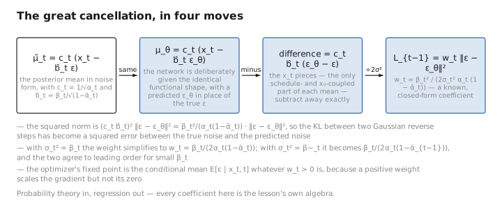
Figure 1. The great cancellation, in four moves.

Weights and signal-to-noise ratio

Define the per-timestep signal-to-noise ratio $\mathrm{SNR}(t)=\bar\alpha_t/(1-\bar\alpha_t)$, the ratio of signal power to noise power in $x_t=\sqrt{\bar\alpha_t}x_0+\sqrt{1-\bar\alpha_t}\,\epsilon$. The variational weight is naturally expressed in these terms. With $\sigma_t^2=\beta_t$,

For the variance-preserving schedule, Kingma et al. (2021) show the continuous-time ELBO contribution of each noise level is proportional to $-\tfrac{d}{dt}\mathrm{SNR}(t)$ times the $\epsilon$-MSE: the loss is an SNR-weighted denoising score-matching objective, and the discrete $w_t$ above is its finite-difference image. Concretely, $w_t$ is large at small $t$ (high SNR, easy denoising) and small at large $t$ (low SNR, where $x_t$ is nearly pure noise).

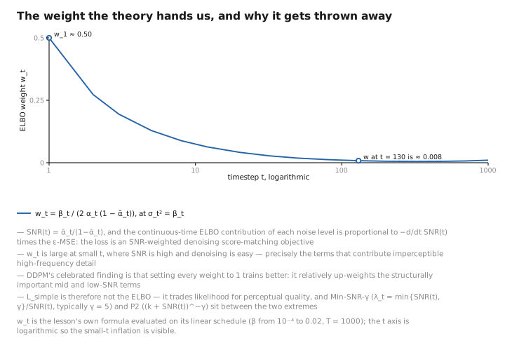
Figure 2. The weight the theory hands us, and why it gets thrown away.

Dropping the weights: the “simple” loss

The exact objective is in hand. What follows is the small heresy that made diffusion work in practice — discarding the very weight the theory just handed us.

DDPM’s celebrated empirical finding is that setting all weights to 1 trains better. Replacing $w_t$ by $1$ down-weights the high-SNR small-$t$ terms — which the ELBO weight inflates but which contribute imperceptible high-frequency detail — and relatively up-weights the structurally important mid/low-SNR terms. The result is the simplified objective:

It compresses the entire training procedure into one expectation:

1. Draw a real image $x_0\sim q$.
2. Draw a timestep $t\sim\mathcal U\{1,\dots,T\}$.
3. Draw noise $\epsilon\sim\mathcal N(0,I)$.
4. Form $x_t=\sqrt{\bar\alpha_t}x_0+\sqrt{1-\bar\alpha_t}\,\epsilon$ in one shot (Lesson 2’s closed-form marginal).
5. Predict $\epsilon_\theta(x_t,t)$.
6. Penalize $\|\epsilon-\epsilon_\theta\|^2$; backpropagate; repeat.

No adversary, no sequential rollout, no intractable normalizer — a regression problem with infinite, free-to-generate training pairs. Each $(x_0,t,\epsilon)$ triple yields a fresh $(x_t,\epsilon)$ example, and the unbiased single-sample Monte-Carlo estimate of the expectation is exactly the per-minibatch loss.

Remark (likelihood vs. quality; min-SNR-$\gamma$). $L_{\text{simple}}$ is not the ELBO: maximizing it does not maximize $\log p_\theta(x_0)$. It trades likelihood (which the true weighting $w_t$ optimizes) for FID/perceptual quality. The two regimes can be reconciled by choosing a weighting $\lambda_t$ between the extremes. Min-SNR-$\gamma$ (Hang et al., 2023) sets $\lambda_t=\min\{\mathrm{SNR}(t),\gamma\}/\mathrm{SNR}(t)$ in $x_0$-space (typically $\gamma=5$), which clamps the otherwise unbounded high-SNR contribution and accelerates convergence; P2 weighting (Choi et al., 2022) uses $\lambda_t=(k+\mathrm{SNR}(t))^{-\gamma}$ to concentrate capacity on the “content-bearing” middle noise levels. $L_{\text{simple}}$ ($\lambda_t\equiv 1$ in $\epsilon$-space), the ELBO ($\lambda_t=w_t$), Min-SNR, and P2 are all instances of the same family $\sum_t \lambda_t\,\mathbb E\|\epsilon-\epsilon_\theta\|^2$; only the per-$t$ emphasis differs. Since each is a positive reweighting of the same nonnegative per-$t$ MSE, all share the same global minimizer $\epsilon_\theta(x_t,t)=\mathbb E[\epsilon\mid x_t,t]$; the weighting governs optimization dynamics and the implicit objective under finite capacity, not the idealized optimum.

Why predicting noise (not the image) works so well

• Scale stability. $\epsilon$ has unit variance at every $t$, so the regression target is consistently scaled across timesteps — gentle on the optimizer and on weight-decay/learning-rate choices. The $x_0$-target, by contrast, is implicitly divided by $\sqrt{1-\bar\alpha_t}$ relative to the $\epsilon$-target (see the linear maps below), so its effective training-target variance blows up as $\bar\alpha_t\to 1$ (small $t$) and collapses as $\bar\alpha_t\to 0$ (large $t$).
• Connection to denoising score matching. As shown in Lesson 9, $\epsilon_\theta(x_t,t)\approx -\sqrt{1-\bar\alpha_t}\,\nabla_{x_t}\log q(x_t)$, i.e. predicting noise is (up to the schedule factor) estimating the score. $L_{\text{simple}}$ is thus a weighted denoising-score-matching objective.
• Empirics. It produces sharper, better samples than the $x_0$- or $\mu$-targets in the original DDPM study.

Equivalent targets, same model: the exact linear maps

Given $x_t$ and $t$, the quantities $x_0$, $\epsilon$, and the velocity $v$ are mutually affine. Fix $\sqrt{\bar\alpha_t}$ and $\sqrt{1-\bar\alpha_t}$. From the forward marginal,

The $v$-parameterization (Salimans & Ho, 2022) defines

which inverts (using $\bar\alpha_t+(1-\bar\alpha_t)=1$) to

Equivalently, with angle $\phi_t$ such that $\cos\phi_t=\sqrt{\bar\alpha_t}$, $\sin\phi_t=\sqrt{1-\bar\alpha_t}$, the map $(x_0,\epsilon)\mapsto(x_t,v)$ is a rotation by $\phi_t$; $v$ is the velocity $dx_t/d\phi_t$ along the diffusion arc, and is the target of choice for stability near both endpoints and for distillation. Predicting any one target and converting to another at sampling time is exact:

Remark (target-variance scaling). Under $x_t=\cos\phi_t\,x_0+\sin\phi_t\,\epsilon$, the three targets have marginal scales $\mathrm{Var}(\epsilon)=1$ (constant), $\mathrm{Var}(x_0)$ fixed by the data, and $\mathrm{Var}(v)=\cos^2\phi_t\cdot 1+\sin^2\phi_t\cdot\mathrm{Var}(x_0)$, which interpolates smoothly between the two endpoints. This is why $\epsilon$-prediction is well-conditioned at high noise, $x_0$-prediction at low noise, and $v$-prediction across the whole range — a fact that the EDM preconditioning (Lesson 6/Karras et al., 2022) formalizes by scaling inputs, targets, and skip weights so the network always sees a unit-variance regression problem.

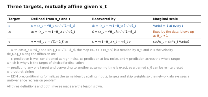
Figure 3. Three targets, mutually affine given x_t.

Code: the simple loss with optional SNR weighting

import torch
import torch.nn.functional as F

def diffusion_loss(model, x0, alpha_bar, weighting="simple", gamma=5.0):
    """
    model:     eps_theta(x_t, t) -> predicted noise, shape (B, C, H, W)
    x0:        clean batch, shape (B, C, H, W)
    alpha_bar: precomputed cumulative products, shape (T,) on x0.device
    weighting: "simple" (lambda_t = 1), "snr", or "min_snr"
    """
    B = x0.shape[0]
    T = alpha_bar.shape[0]
    t = torch.randint(0, T, (B,), device=x0.device)        # (B,)
    ab = alpha_bar[t].view(B, 1, 1, 1)                      # (B,1,1,1) broadcast

    eps = torch.randn_like(x0)                              # (B,C,H,W)
    x_t = ab.sqrt() * x0 + (1.0 - ab).sqrt() * eps          # forward marginal, one shot
    eps_pred = model(x_t, t)                                # (B,C,H,W)

    # per-example MSE, averaged over C,H,W -> shape (B,)
    se = F.mse_loss(eps_pred, eps, reduction="none").flatten(1).mean(1)

    if weighting == "simple":
        w = torch.ones_like(se)
    else:
        snr = ab / (1.0 - ab)                               # (B,1,1,1)
        snr = snr.flatten()                                 # (B,)
        if weighting == "snr":
            w = snr                                         # ELBO-like (eps-space ~ const; x0-space ~ snr)
        elif weighting == "min_snr":
            w = torch.clamp(snr, max=gamma) / snr           # Min-SNR-gamma in eps-space
        w = w.detach()                                      # weighting must not receive gradient

    return (w * se).mean()

Numerical notes. Precompute alpha_bar in float64 then cast, since $\bar\alpha_t=\prod_{s\le t}(1-\beta_s)$ underflows toward $0$ at large $t$ for $T\sim 1000$. Clamp $1-\bar\alpha_t$ away from $0$ (e.g. $\ge 10^{-5}$) before .sqrt() at $t=0$ to avoid division by zero in $\hat x_0$. Detach the weights so gradients flow only through eps_pred. The reduction="none" + per-example mean keeps the loss scale independent of resolution.

Exercises

Throughout, use the lesson’s local shorthand $c_t:=1/\sqrt{\alpha_t}$ and $\hat b_t:=\beta_t/\sqrt{1-\bar\alpha_t}$, so $\tilde\mu_t=c_t(x_t-\hat b_t\epsilon)$ and $\mu_\theta=c_t(x_t-\hat b_t\epsilon_\theta)$.

1. The cancellation. Show $\|\tilde\mu_t-\mu_\theta\|^2=(c_t\hat b_t)^2\|\epsilon-\epsilon_\theta\|^2=\frac{\beta_t^2}{\alpha_t(1-\bar\alpha_t)}\|\epsilon-\epsilon_\theta\|^2$.

$\tilde\mu_t-\mu_\theta=c_t[(x_t-\hat b_t\epsilon)-(x_t-\hat b_t\epsilon_\theta)]=c_t\hat b_t(\epsilon_\theta-\epsilon)$ — the $x_t$ pieces (the only schedule/$x_0$-coupled parts) cancel exactly. Squaring, $\|\tilde\mu_t-\mu_\theta\|^2=(c_t\hat b_t)^2\|\epsilon-\epsilon_\theta\|^2$, and $(c_t\hat b_t)^2=\frac{1}{\alpha_t}\cdot\frac{\beta_t^2}{1-\bar\alpha_t}=\frac{\beta_t^2}{\alpha_t(1-\bar\alpha_t)}$.

2. The weight under $\sigma_t^2=\tilde\beta_t$. Dividing by $2\sigma_t^2$ defines $w_t=\frac{\beta_t^2}{2\sigma_t^2\alpha_t(1-\bar\alpha_t)}$. Simplify $w_t$ when $\sigma_t^2=\tilde\beta_t=\frac{1-\bar\alpha_{t-1}}{1-\bar\alpha_t}\beta_t$.

3. Same optimum for any positive weighting. Show that for any weights $\lambda_t\gt 0$, the objective $\sum_t\lambda_t\,\mathbb E\|\epsilon-\epsilon_\theta(x_t,t)\|^2$ is minimized by the same predictor $\epsilon_\theta(x_t,t)=\mathbb E[\epsilon\mid x_t,t]$.

Each per-$t$ term $\mathbb E\|\epsilon-\epsilon_\theta(x_t,t)\|^2$ is an MSE, minimized pointwise (for each $x_t$) by the conditional mean $\mathbb E[\epsilon\mid x_t,t]$ — the standard fact that the minimizer of $\mathbb E\|Y-g(X)\|^2$ is $g(X)=\mathbb E[Y\mid X]$. A positive weight $\lambda_t$ scales a term but does not move its minimizer, and (with enough capacity) all per-$t$ minimizers can be achieved simultaneously, so the weighted sum shares the same global minimizer. The weighting changes only finite-capacity dynamics and the implicit objective, not the idealized optimum.

4. The $v$ inverse map. Verify that $v:=\sqrt{\bar\alpha_t}\,\epsilon-\sqrt{1-\bar\alpha_t}\,x_0$ inverts to $\epsilon=\sqrt{1-\bar\alpha_t}\,x_t+\sqrt{\bar\alpha_t}\,v$, using $x_t=\sqrt{\bar\alpha_t}\,x_0+\sqrt{1-\bar\alpha_t}\,\epsilon$ and $\bar\alpha_t+(1-\bar\alpha_t)=1$.

Write $a_t=\sqrt{\bar\alpha_t},\,b_t=\sqrt{1-\bar\alpha_t}$ (so $a_t^2+b_t^2=1$). Then

Conclusion

The $\epsilon$-parameterization gives $\mu_\theta$ the same functional form as $\tilde\mu_t$, so the $x_t$ terms cancel exactly and the Gaussian KL collapses to $w_t\|\epsilon-\epsilon_\theta\|^2$ with $w_t=\frac{\beta_t^2}{2\sigma_t^2\alpha_t(1-\bar\alpha_t)}$. Replacing $w_t$ by $1$ yields the simplified DDPM loss $L_{\text{simple}}=\mathbb E\,\|\epsilon-\epsilon_\theta(x_t,t)\|^2$ — a stable, unit-variance-target regression with an endless supply of training pairs, sitting in a one-parameter-family of SNR weightings (ELBO, Min-SNR-$\gamma$, P2) that all share the same optimum but differ in finite-capacity dynamics and the likelihood-vs-quality tradeoff. The $\epsilon$-, $x_0$-, and $v$-targets are exact affine images of one another given $x_t$. In Lesson 6 we open the box labeled $\epsilon_\theta$: the U-Net architecture, how the timestep $t$ is injected, and why this network shape suits denoising.

All that apparatus folded into three words: guess the noise. The objective is as simple as it will ever be, and infinitely supplied with training pairs. In Lesson 6 we finally lift the lid on the thing doing the guessing — the network $\epsilon_\theta$ we have invoked for five lessons without once describing.

References

• J. Ho, A. Jain, P. Abbeel. Denoising Diffusion Probabilistic Models. NeurIPS 2020. (The $\epsilon$-parameterization, the cancellation, and $L_{\text{simple}}$.)
• D. P. Kingma, T. Salimans, B. Poole, J. Ho. Variational Diffusion Models. NeurIPS 2021. (Continuous-time ELBO as SNR-weighted denoising; the role of $\mathrm{SNR}(t)$.)
• T. Salimans, J. Ho. Progressive Distillation for Fast Sampling of Diffusion Models. ICLR 2022. (The $v$-parameterization and its rotation geometry.)
• T. Hang, S. Gu, C. Li, et al. Efficient Diffusion Training via Min-SNR Weighting Strategy. ICCV 2023. (Min-SNR-$\gamma$ reweighting.)
• J. Choi, J. Lee, C. Shin, et al. Perception Prioritized Training of Diffusion Models (P2). CVPR 2022. (P2 SNR-based weighting and the content-bearing noise levels.)

← Previous: Lesson 4 — The Variational Lower Bound · Course Index · Next: Lesson 6 — The U-Net Architecture → · Appendix A: Acronyms · Appendix B: Formulas

The figures in this lesson follow the shared figure key , which explains what every shape, line style and colour means.