Lesson 6 — The Network: U-Net and Time Conditioning

Recap of Lesson 5. The $\epsilon$-parameterization $\mu_\theta = \frac{1}{\sqrt{\alpha_t}}(x_t - \frac{\beta_t}{\sqrt{1-\bar\alpha_t}}\epsilon_\theta)$ makes schedule factors cancel, collapsing the variational objective into the simple loss $L_{\text{simple}} = \mathbb E_{t,x_0,\epsilon}\,\|\epsilon - \epsilon_\theta(\sqrt{\bar\alpha_t}x_0+\sqrt{1-\bar\alpha_t}\epsilon,\,t)\|^2$. The network is a noise predictor with unlimited, cheaply-generated training pairs. This lesson opens the box: what is $\epsilon_\theta$ actually made of?

We have spent five lessons describing a job without once meeting the worker who does it: take a noisy image, hand back the noise hidden inside it, and do so at every level of corruption with the same pair of hands. This lesson opens the box we have only ever named by its task. Inside is not a featureless slab but a particular, well-argued shape — a network that narrows until it can see the whole picture at a glance, widens again to put the grain back, and ferries fine detail across the gap on dedicated wires — and that is told, every time, exactly how noisy the image before it is.

Overview

$\epsilon_\theta$ must map an $H\times W\times C$ tensor to an $H\times W\times C$ tensor of the same shape — it is a dense prediction network, not a classifier — while reasoning across spatial scales, since noise corrupts fine texture and coarse structure alike. The U-Net satisfies both constraints: a contracting encoder builds global context at low resolution, an expanding decoder restores spatial precision, and skip connections carry high-frequency detail across the bottleneck. A single shared $\theta$ must denoise at every noise level, so the network is additionally conditioned on $t$ through a sinusoidal embedding fed into a small MLP and broadcast into every block as a learned scale-and-shift. We make the block composition, attention placement and cost, time-conditioning equations, and the U-Net-vs-DiT distinction precise, with correct PyTorch-style code and tensor shapes.

Why image-to-image, and why multi-scale

The target $\epsilon$ lives in the same space as $x_t$ — one value per pixel-channel — so $\epsilon_\theta$ resembles a segmentation network, not a classifier. Denoising is inherently multi-scale: recovering a face needs local cues (edges, grain) and global ones (this region is an eye, hence dark). The contracting path captures global context cheaply at low resolution; the expanding path restores spatial precision; skip connections prevent fine detail from being destroyed at the bottleneck. The same translation-equivariance argument that motivates convolutions for natural images applies here.

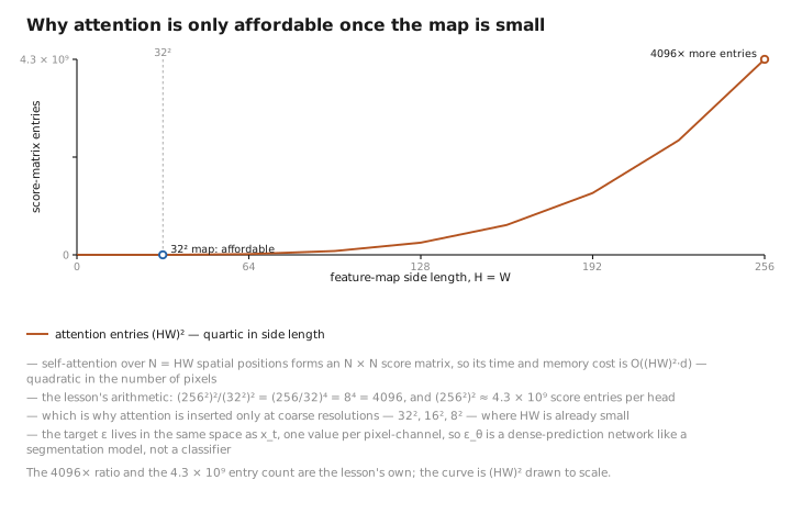
Figure 1. Why attention is only affordable once the map is small.

Anatomy of the U-Net

A diffusion U-Net is a stack of stages at decreasing then increasing resolution:

• Encoder (downsampling path). Repeated residual blocks followed by downsampling. Channel width grows as resolution shrinks to keep per-stage compute and representational capacity roughly balanced, e.g. $256^2\!\times\!128 \to 128^2\!\times\!256 \to 64^2\!\times\!512 \to 32^2\!\times\!512$. A common width rule is a base channel count $C_0$ times a tuple of multipliers, e.g. $C_0\cdot(1,2,4,4)$.
• Bottleneck. Residual + self-attention + residual at the lowest resolution, where the receptive field covers the whole image at low token count.
• Decoder (upsampling path). Mirror of the encoder; each stage upsamples and concatenates the matching encoder feature map via a skip connection before its residual blocks (so the first conv of a decoder block sees $2\times$ the channels).
• Output head. GroupNorm → SiLU → final $3\times3$ conv to $C$ channels — the predicted $\hat\epsilon$ (or $\hat x_0$, or $v$). This last conv is often zero-initialized so the network starts as the identity-noise predictor.

Residual blocks. Each block is GroupNorm → SiLU → Conv(3×3) → (add time projection) → GroupNorm → SiLU → Dropout → Conv(3×3), with the input added back through a skip (a $1\times1$ conv on the skip if channel counts differ):

GroupNorm (not BatchNorm) is used because diffusion batches are small and the statistics must be batch-independent; SiLU/Swish is the standard activation. Residual connections keep gradients healthy through depth.

Self-attention placement and cost. Convolutions have a bounded receptive field; self-attention lets distant regions coordinate, which is necessary for globally coherent samples. Attention over a feature map of $N=HW$ spatial positions forms an $N\times N$ score matrix, so its time and memory cost is

quadratic in the number of pixels. This is why attention is inserted only at coarse resolutions (e.g. $32^2$, $16^2$, $8^2$), where $HW$ is small; placing it at $256^2$ would cost $(256^2)^2\approx 4.3\times 10^9$ score entries per head. Improved diffusion architectures (Nichol & Dhariwal 2021; Dhariwal & Nichol 2021) use multi-head attention at multiple low resolutions, more residual blocks per stage, and BigGAN-style up/down residual blocks, finding these scale the model favorably.

Down/upsampling choices. Downsampling is a stride-2 convolution (learned) or average pooling; upsampling is nearest-neighbor interpolation followed by a $3\times3$ conv (preferred over transposed conv, which produces checkerboard artifacts). Parameter count is dominated by the wide low-resolution stages and the bottleneck attention; FLOPs are dominated by the high-resolution stages, motivating the channel-growth schedule above.

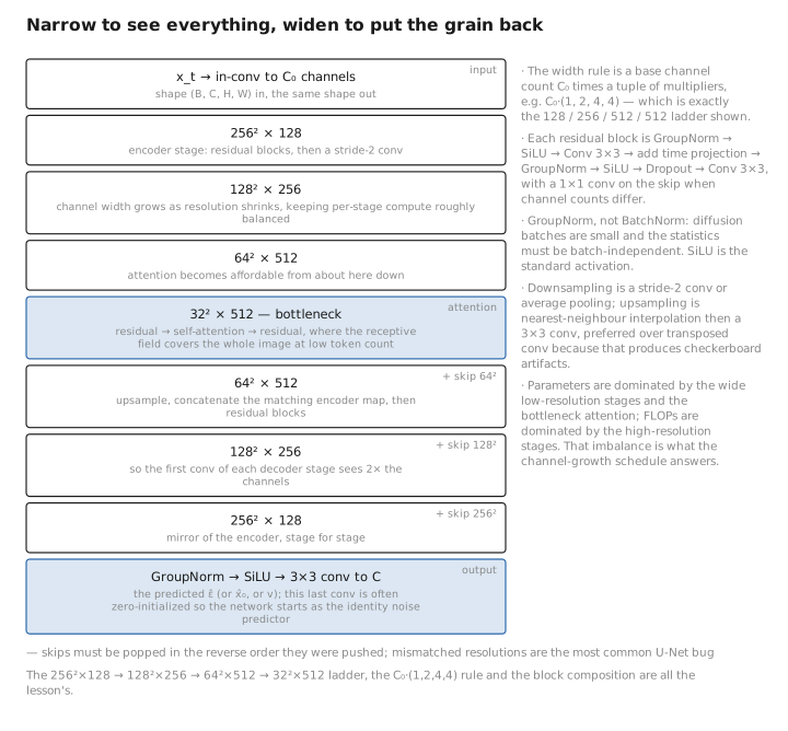
Figure 2. Narrow to see everything, widen to put the grain back.

Injecting the timestep $t$

A single set of weights must serve a thousand different noise levels, which raises the obvious question: how does the network know which level it is looking at?

The shared weights must denoise at every noise level, so the network needs to know $t$. We do not feed the raw integer; we build a smooth, high-dimensional embedding.

Step 1 — sinusoidal embedding. Map the scalar $t$ to a vector of sines and cosines at geometrically spaced frequencies (Vaswani et al., 2017):

The geometric frequency ladder spans wavelengths from $2\pi$ to $2\pi\cdot 10000$, so coarse and fine differences in $t$ are simultaneously representable. The construction is motivated by linearity: for a fixed offset $\delta$, $\text{emb}(t+\delta)$ is a fixed linear (rotation) function of $\text{emb}(t)$, since $\sin(\omega(t+\delta))$ and $\cos(\omega(t+\delta))$ are linear combinations of $\sin(\omega t),\cos(\omega t)$. The network can therefore read off relative noise level via a linear map, and nearby timesteps map to nearby vectors (Lipschitz in $t$), which raw one-hot or integer inputs would not provide.

Step 2 — small MLP. Pass $\text{emb}(t)$ through a two-layer MLP with a nonlinearity to produce the conditioning vector $\tau \in \mathbb R^{d_\tau}$:

Step 3 — FiLM / adaLN scale-shift injection. Inside each residual block, $\tau$ is projected to the block’s channel count $C$ and used to modulate the normalized features. The simplest form is an additive bias (FiLM with unit scale; Perez et al., 2018), $h\leftarrow h + W_\tau\tau$, broadcast over $H,W$. The more expressive and now-standard form is a per-channel scale-and-shift applied to a normalized activation:

with $\gamma,\beta\in\mathbb R^{C}$ broadcast over spatial dimensions. This is FiLM/adaptive-GroupNorm in the U-Net and adaLN in transformers. Writing $1+\gamma$ rather than $\gamma$ centers the modulation at identity, so zero-initializing $W_\tau$ makes each block start as an unconditioned residual block and learn conditioning gradually (the “Zero” variant; see DiT below).

A more complete forward-pass sketch

import math, torch, torch.nn as nn, torch.nn.functional as F

def sinusoidal_embedding(t, dim):
    # t: (B,) integer or float timesteps  ->  (B, dim)
    half = dim // 2
    freqs = torch.exp(-math.log(10000) * torch.arange(half, device=t.device) / half)
    args = t[:, None].float() * freqs[None, :]          # (B, half)
    return torch.cat([torch.sin(args), torch.cos(args)], dim=-1)  # (B, dim)

class ResBlock(nn.Module):
    def __init__(self, c_in, c_out, t_dim):
        super().__init__()
        self.norm1 = nn.GroupNorm(32, c_in)
        self.conv1 = nn.Conv2d(c_in, c_out, 3, padding=1)
        self.t_proj = nn.Linear(t_dim, 2 * c_out)        # -> (gamma, beta)
        self.norm2 = nn.GroupNorm(32, c_out)
        self.conv2 = nn.Conv2d(c_out, c_out, 3, padding=1)
        self.skip = nn.Conv2d(c_in, c_out, 1) if c_in != c_out else nn.Identity()

    def forward(self, h, tau):                           # h:(B,c_in,H,W) tau:(B,t_dim)
        x = self.conv1(F.silu(self.norm1(h)))            # (B,c_out,H,W)
        gamma, beta = self.t_proj(tau).chunk(2, dim=1)   # each (B,c_out)
        x = self.norm2(x)
        x = (1 + gamma[:, :, None, None]) * x + beta[:, :, None, None]   # adaGN scale-shift
        x = self.conv2(F.silu(x))                        # (B,c_out,H,W)
        return x + self.skip(h)

class AttnBlock(nn.Module):                              # self-attention over HW tokens
    def __init__(self, c, heads=4):
        super().__init__()
        self.norm = nn.GroupNorm(32, c)
        self.qkv = nn.Conv2d(c, 3 * c, 1)
        self.proj = nn.Conv2d(c, c, 1)
        self.heads = heads

    def forward(self, h):                                # h:(B,C,H,W)
        B, C, H, W = h.shape
        q, k, v = self.qkv(self.norm(h)).chunk(3, dim=1) # each (B,C,H,W)
        # reshape to (B, heads, HW, C/heads)
        resh = lambda z: z.reshape(B, self.heads, C // self.heads, H * W).transpose(-1, -2)
        out = F.scaled_dot_product_attention(resh(q), resh(k), resh(v))   # O((HW)^2)
        out = out.transpose(-1, -2).reshape(B, C, H, W)
        return h + self.proj(out)                        # residual

class UNet(nn.Module):
    def __init__(self, c_img=3, c0=128, mults=(1, 2, 4, 4), t_dim=512, attn_res={16, 8}):
        super().__init__()
        self.t_mlp = nn.Sequential(nn.Linear(c0, t_dim), nn.SiLU(), nn.Linear(t_dim, t_dim))
        self.c0 = c0
        # ... encoder ResBlocks/AttnBlocks/Downsample, bottleneck, decoder mirrored ...
        # encoder stages append feature maps to `skips`; decoder concatenates them.
        self.in_conv = nn.Conv2d(c_img, c0, 3, padding=1)
        self.out = nn.Sequential(nn.GroupNorm(32, c0), nn.SiLU(),
                                 nn.Conv2d(c0, c_img, 3, padding=1))   # zero-init last conv

    def forward(self, x_t, t):                           # x_t:(B,C,H,W) t:(B,)
        tau = self.t_mlp(sinusoidal_embedding(t, self.c0))            # (B, t_dim)
        h = self.in_conv(x_t)
        skips = [h]
        # for stage in encoder:  h = resblock(h, tau); (attn if H in attn_res); skips.append(h); h = downsample(h)
        # h = bottleneck_res2(attn(bottleneck_res1(h, tau)), tau)
        # for stage in decoder:  h = upsample(h); h = cat([h, skips.pop()], 1); h = resblock(h, tau)
        return self.out(h)                               # (B,C,H,W) predicted noise

scaled_dot_product_attention makes the $O((HW)^2)$ cost explicit and uses a fused/flash kernel when available. Use GroupNorm(32, c) with c divisible by 32; zero-initialize the final conv and each block’s t_proj for stable early training. Skips must be popped in the reverse order they were pushed; mismatched resolutions are the most common U-Net bug.

U-Net vs. Diffusion Transformer (DiT)

None of the framework so far cares that the worker happens to be a U-Net; to prove the point, we now swap the worker out entirely and watch the loss and loop stay put.

The framework of Lessons 1–5 is architecture-agnostic — only $\epsilon_\theta$ changes. The Diffusion Transformer (Peebles & Xie, 2023) replaces the convolutional U-Net with a plain transformer on a (latent) image:

• Patchify. Split the $h\times w\times c$ latent into non-overlapping $p\times p$ patches and linearly embed each into a $D$-dimensional token, giving $N=(h/p)(w/p)$ tokens. Smaller $p$ means more tokens, higher cost, finer detail.
• Positional + time embeddings. Add (sinusoidal or learned) 2-D positional embeddings to the tokens. The timestep $t$ (and any class/text condition $c$) are embedded and supplied not as tokens but as conditioning to adaLN.
• adaLN-Zero. Each transformer block replaces LayerNorm’s affine parameters with $\gamma,\beta$ regressed from $\tau$ (the embedded $t,c$), exactly the scale-shift of the U-Net but on token features, plus a learned residual gate $\alpha$: $h\leftarrow h+\alpha\odot\mathrm{Block}((1+\gamma)\,\mathrm{LN}(h)+\beta)$. The gate and the modulation MLP are zero-initialized so each block starts as the identity — the “Zero” in adaLN-Zero — which is what makes deep DiTs trainable.
• Unpatchify. A final linear layer maps each token back to a $p\times p\times c$ patch; reassemble into the output grid.

Same loss, same training loop, same $(x_t,t)\mapsto\hat\epsilon$ signature. DiT trades the U-Net’s built-in multi-scale inductive bias (downsampling + skips) for global self-attention at every layer and clean scaling with compute; it is the backbone of recent large text-to-image and video systems. Both designs can be combined with EDM-style preconditioning (Karras et al., 2022), which rescales the network’s input, output, and skip so it always solves a unit-variance regression regardless of noise level (cf. Lesson 5’s target-variance remark).

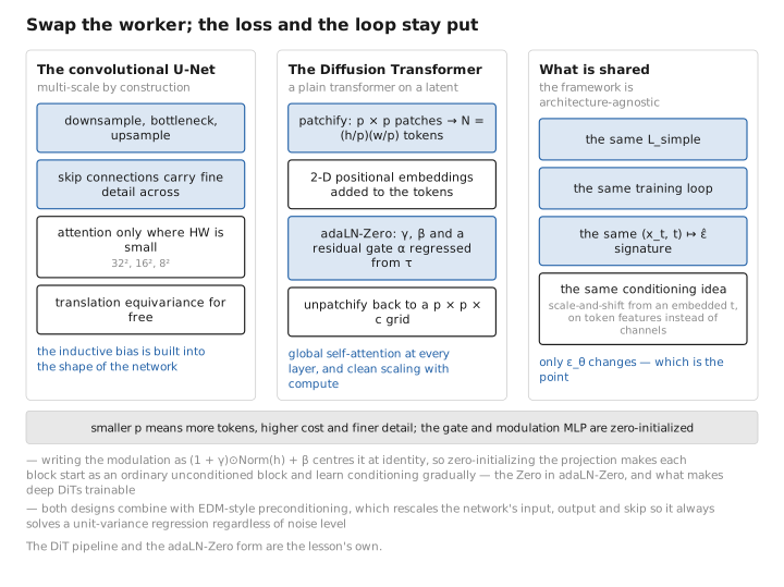
Figure 3. Swap the worker; the loss and the loop stay put.

Exercises

1. Why attention only at coarse resolutions. Self-attention over an $H\times W$ feature map forms an $N\times N$ score matrix with $N=HW$, costing $O((HW)^2)$. Compute the ratio of score-matrix entries between a $256\times256$ map and a $32\times32$ map, and use it to justify placing attention only at low resolution.

$\dfrac{(256^2)^2}{(32^2)^2}=\left(\dfrac{256}{32}\right)^4=8^4=4096$. The full-resolution map needs $\sim\!4096\times$ as many score entries (and as much attention compute/memory) as the $32^2$ map — prohibitive — which is why attention is inserted only where $HW$ is already small.

2. Linearity of the sinusoidal embedding. Show that for a fixed offset $\delta$, the pair $(\sin\omega t,\cos\omega t)$ is mapped to $(\sin\omega(t+\delta),\cos\omega(t+\delta))$ by a rotation matrix that does not depend on $t$.

By the angle-addition formulas,

The matrix depends only on $\omega\delta$, not on $t$ — so $\text{emb}(t+\delta)$ is a fixed linear (rotation) function of $\text{emb}(t)$, letting the network read relative timestep shifts with a linear map.

3. Identity-at-init modulation. Explain why the scale-shift is written $(1+\gamma)\odot\mathrm{Norm}(h)+\beta$ rather than $\gamma\odot\mathrm{Norm}(h)+\beta$, and what zero-initializing the projection that produces $(\gamma,\beta)$ achieves.

With the projection zero-initialized, $\gamma=\beta=0$, so the modulation becomes $(1+0)\odot\mathrm{Norm}(h)+0=\mathrm{Norm}(h)$ — the identity transform. The block therefore starts as an ordinary, unconditioned residual block and learns conditioning gradually, which stabilizes early training (the “Zero” in adaLN-Zero). Writing plain $\gamma$ would zero out the activations at init instead.

4. Decoder channel doubling. Why does the first convolution of a decoder stage receive $2C$ input channels when the stage works at width $C$?

Each decoder stage concatenates the matching encoder feature map (via the skip connection) with the upsampled decoder feature along the channel axis — $C$ channels from each — giving $2C$. The first conv must therefore accept $2C$ inputs. (Popping skips in the wrong order, or mismatched resolutions, is the most common U-Net bug.)

Conclusion

The noise predictor $\epsilon_\theta$ is an image-to-image U-Net: residual blocks of GroupNorm → SiLU → Conv with adaptive scale-shift time injection, self-attention at coarse resolutions (paying its $O((HW)^2)$ cost only where $HW$ is small), learned down/up-sampling, and skip connections matched to the multi-scale nature of denoising. The timestep enters as a sinusoidal embedding → MLP → per-block FiLM/adaLN scale-shift, justified by the linearity of sinusoids under timestep offsets, so one shared network denoises at every level. The DiT keeps the loss and loop but swaps the convolutional backbone for a transformer with patchify, positional+time embeddings, adaLN-Zero conditioning, and unpatchify. We now have the loss (Lesson 5) and the machine that computes it (this lesson). In Lesson 7 we assemble them into the complete, runnable training algorithm.

The box is open, and the worker turns out to be a sensible machine rather than a mystery. We now have the objective (Lesson 5) and the apparatus that computes it (this lesson). Lesson 7 puts the two on the same bench and writes the loop that actually trains them.

References

• O. Ronneberger, P. Fischer, T. Brox. U-Net: Convolutional Networks for Biomedical Image Segmentation. MICCAI 2015. (Encoder–decoder with skip connections.)
• J. Ho, A. Jain, P. Abbeel. Denoising Diffusion Probabilistic Models. NeurIPS 2020. (U-Net backbone with sinusoidal time embedding and attention.)
• A. Nichol, P. Dhariwal. Improved Denoising Diffusion Probabilistic Models. ICML 2021. (Architecture/attention/cosine-schedule improvements.)
• P. Dhariwal, A. Nichol. Diffusion Models Beat GANs on Image Synthesis. NeurIPS 2021. (Improved U-Net: multi-resolution attention, more blocks, BigGAN up/down.)
• A. Vaswani, et al. Attention Is All You Need. NeurIPS 2017. (Sinusoidal positional embeddings; scaled dot-product attention.)
• E. Perez, F. Strub, H. de Vries, V. Dumoulin, A. Courville. FiLM: Visual Reasoning with a General Conditioning Layer. AAAI 2018. (Feature-wise scale-shift conditioning.)
• W. Peebles, S. Xie. Scalable Diffusion Models with Transformers (DiT). ICCV 2023. (Patchify, adaLN-Zero, unpatchify.)
• T. Karras, M. Aittala, T. Aila, S. Laine. Elucidating the Design Space of Diffusion-Based Generative Models (EDM). NeurIPS 2022. (Input/output/skip preconditioning.)

← Previous: Lesson 5 — The Simplified Objective · Course Index · Next: Lesson 7 — The Training Algorithm → · Appendix A: Acronyms · Appendix B: Formulas

The figures in this lesson follow the shared figure key , which explains what every shape, line style and colour means.