Lesson 7 — The Training Algorithm in Practice

Recap of Lesson 6. The noise predictor $\epsilon_\theta$ is an image-to-image U-Net — contracting encoder, attention bottleneck, expanding decoder, skip connections — with the timestep injected via a sinusoidal embedding passed through an MLP and added (as scale/shift) inside every residual block. Modern systems may use a Diffusion Transformer instead, but the loss is unchanged. This lesson assembles the loss and the network into the full training phase.

Everything so far has been scaffolding — the forward jump, the tractable posterior, the bound, the great cancellation — and scaffolding can trick you into expecting an elaborate building. Here is the building. It fits on an index card: sample an image, pick a noise level, add noise, ask the network to name it, nudge the weights. Five lines. The rest of this lesson is about taking that humble loop seriously enough to make it converge to a competitive model — and about the one thing it conspicuously refuses to do.

Overview

Every result from Lessons 2–5 collapses into a loop that fits on an index card. The closed-form forward jump $q(x_t\mid x_0)$, the tractable posterior $q(x_{t-1}\mid x_t,x_0)$, the variational bound, and the algebraic cancellation of the KL terms into a noise-prediction MSE all exist to make this loop trivial: at no point does training simulate the reverse chain. Each gradient step performs a single one-shot noising and a single network evaluation per example. The cost asymmetry that defines diffusion — cheap training, expensive sampling — originates here.

The training algorithm (DDPM)

repeat

1. $x_0 \sim q(x_0)$    — sample a minibatch of real data
2. $t \sim \mathcal{U}\{1, \dots, T\}$    — sample a timestep per example, uniformly
3. $\epsilon \sim \mathcal{N}(0, I)$    — sample noise, same shape as $x_0$
4. $x_t = \sqrt{\bar\alpha_t}\,x_0 + \sqrt{1-\bar\alpha_t}\,\epsilon$    — one-shot forward jump (Lesson 2)
5. Take a gradient step on $\nabla_\theta \big\|\epsilon - \epsilon_\theta(x_t, t)\big\|^2$

until converged

Five lines, no adversary, no reverse rollout, no likelihood normalizer. The remainder of the lesson treats this loop as what it is: a doubly-stochastic Monte-Carlo estimator of the variational objective, and analyzes its bias, variance, and the engineering required to make it converge to a competitive model.

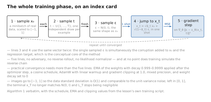
Figure 1. The whole training phase, on an index card.

The loop as a Monte-Carlo estimator

The loop is short enough to memorize in a minute; understanding why it is correct — why five lines faithfully estimate a sum over a thousand KL terms — takes a little more care.

From the variational bound to $L_\text{simple}$

Lesson 4 decomposed the negative ELBO into a sum of per-timestep KL terms,

$$ \mathcal L_\text{vlb} = \underbrace{D_{\mathrm{KL}}!\big(q(x_T\mid x_0),|,p(x_T)\big)}_{L_T}

• \sum_{t=2}^{T}\underbrace{D_{\mathrm{KL}}!\big(q(x_{t-1}\mid x_t,x_0),|,p_\theta(x_{t-1}\mid x_t)\big)}{L{t-1}} ;\underbrace{-,\log p_\theta(x_0\mid x_1)}_{L_0}. $$

With Gaussian $p_\theta$ of fixed variance and the $\epsilon$-parameterization, each $L_{t-1}$ reduces to a weighted noise-prediction MSE,

Ho et al. (2020) observed empirically that dropping the weight ($w_t\equiv 1$) improves sample quality, yielding the simple objective in line 5:

Unbiasedness and variance of the estimator

The loop never forms $\sum_t L_{t-1}$ explicitly. Instead, at each step it draws a single triple $(x_0,t,\epsilon)$ and evaluates $g=\big\|\epsilon-\epsilon_\theta(x_t,t)\big\|^2$. Because $t$ is uniform on $\{1,\dots,T\}$,

so the per-sample gradient $\nabla_\theta g$ is an unbiased estimator of $\nabla_\theta L_\text{simple}$ up to the constant $1/T$ absorbed into the learning rate. Minibatching of size $B$ averages $B$ such i.i.d. draws, reducing the estimator variance by $1/B$ in the usual way. The two sources of stochasticity — the data/noise draw $(x_0,\epsilon)$ and the timestep draw $t$ — both inflate gradient variance, and the timestep variance is the one we can cheaply reshape.

Remark (importance sampling over $t$). Replace uniform sampling by a proposal $t\sim p(t)$ and reweight: with $p(t)\propto \mathbb{E}[L_{t-1}]$ optimal, the estimator

$$\hat L = \frac{1}{p(t)}\,L_{t-1}, \qquad \mathbb{E}_{t\sim p}[\hat L] = \sum_t L_{t-1},$$

remains unbiased for any $p(t)\gt 0$ but attains lower variance when $p(t)$ tracks the per-$t$ loss magnitude. Nichol & Dhariwal (2021) maintain a running estimate of $\mathbb{E}[L_{t-1}^2]$ and set $p(t)\propto\sqrt{\mathbb{E}[L_{t-1}^2]}$, the variance-minimizing choice for an unweighted sum. This is essential when training the full $\mathcal L_\text{vlb}$ (e.g. when learning $\Sigma_\theta$), whose per-$t$ terms span several orders of magnitude.

Remark (Min-SNR weighting). Hang et al. (2023) reframe the choice of $w_t$ as a multi-task balancing problem across noise levels and show that $L_\text{simple}$ ($w_t\equiv1$) over-weights low-noise steps while $\mathcal L_\text{vlb}$ over-weights high-noise steps. Their Min-SNR-$\gamma$ weight,

$$ w_t = \frac{\min\{\mathrm{SNR}(t),\,\gamma\}}{\mathrm{SNR}(t)}, \qquad \mathrm{SNR}(t) = \frac{\bar\alpha_t}{1-\bar\alpha_t}, $$

caps the effective gradient magnitude at high SNR (small $t$) with $\gamma\approx5$, accelerating convergence by 3–4$\times$. For the $\epsilon$-prediction target $w_t$ multiplies the loss directly; for $x_0$- or $v$-prediction the SNR factor enters differently (see the $v$-prediction remark below). Karras et al. (2022) reach the same conclusion from the continuous-time EDM perspective, prescribing a loss weighting $\lambda(\sigma)$ and a log-normal sampling density over noise scales $\sigma$.

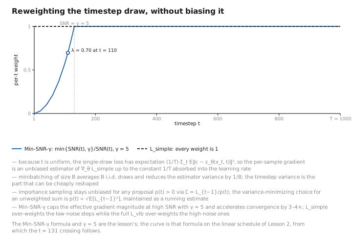
Figure 2. Reweighting the timestep draw, without biasing it.

Line-by-line, with the details that matter

Step 1 — data. Standard minibatching. Images are scaled to $[-1,1]$ so that the empirical data standard deviation is $O(1)$ and comparable to the unit-variance noise; the variance-preserving schedule presumes signal and noise share a scale.

Remark (data scaling and SNR). The forward marginal has variance $\bar\alpha_t\,\mathrm{Var}(x_0) + (1-\bar\alpha_t)$. With $\mathrm{Var}(x_0)\approx1$ this is $\approx1$ for all $t$ (variance-preserving), so $\mathrm{SNR}(t)=\bar\alpha_t/(1-\bar\alpha_t)$ is the only quantity that varies along the chain. If data are not centered and scaled — e.g. left in $[0,1]$ — the terminal $x_T$ no longer matches the standard-normal prior $p(x_T)=\mathcal N(0,I)$, $L_T$ becomes non-negligible, and there is a train/sample prior mismatch. Latent-diffusion pipelines apply an analogous per-channel normalization to the VAE latents (a fixed scaling factor) for the same reason.

Step 2 — sampling $t$. Each example draws an independent $t$, realizing the Monte-Carlo estimate of $\sum_t L_{t-1}$ analyzed above. Uniform sampling corresponds to $L_\text{simple}$; importance sampling or Min-SNR replaces it when variance reduction or rebalancing is needed.

Step 3–4 — corruption in one shot. The single sampled $\epsilon$ is simultaneously (a) the corruption added to $x_0$ and (b) the regression target. They are the same vector — the conceptual core of the method. Using the closed form (Lesson 2) we jump directly to noise level $t$ without simulating intermediate steps.

Step 5 — the gradient. Plain MSE between predicted and true noise, backpropagated through $\epsilon_\theta$. The target is unit-variance and the loss is quadratic, so there is no min-max instability and no mode collapse.

Remark (why we never roll out the reverse chain). The objective minimized is the variational bound, a surrogate that upper-bounds $-\log p_\theta(x_0)$ and decomposes into per-step KL divergences between the tractable posterior $q(x_{t-1}\mid x_t,x_0)$ and the model $p_\theta(x_{t-1}\mid x_t)$. Each term is computed in closed form from a single $x_t$; matching the per-step conditionals is sufficient to control the marginal likelihood. Rolling out the reverse chain (as score-distillation or consistency-style training do) would require backpropagating through $T$ sequential network calls — quadratically more expensive and high-variance — and is provably unnecessary for the ELBO. This is the single most important structural fact of diffusion training.

A complete training script

Theory satisfied, here is what the loop looks like once every practical detail that separates a toy from a trained model has been filled back in.

The fragment below is a self-contained, correct training step including schedule construction (linear and cosine), buffer registration, EMA, AdamW with warmup and gradient clipping, and mixed precision. Tensor shapes are annotated; broadcasting follows PyTorch convention.

import math, copy
import torch
import torch.nn.functional as F
from torch.optim import AdamW
from torch.optim.lr_scheduler import LambdaLR

# ---------- Schedule construction ----------
def linear_beta_schedule(T, beta_start=1e-4, beta_end=2e-2):
    return torch.linspace(beta_start, beta_end, T)                 # (T,)

def cosine_alpha_bar_schedule(T, s=0.008):
    # Nichol & Dhariwal (2021): define alpha_bar directly, then derive betas.
    t = torch.linspace(0, T, T + 1)                               # (T+1,)
    f = torch.cos(((t / T + s) / (1 + s)) * math.pi / 2) ** 2
    alpha_bar = f / f[0]                                          # alpha_bar[0] = 1
    betas = 1 - (alpha_bar[1:] / alpha_bar[:-1])                  # (T,)
    return betas.clamp(max=0.999)                                 # numerical guard

class Diffusion(torch.nn.Module):
    """Holds the schedule as non-trainable buffers (move with .to(device),
    save with state_dict, never receive gradients)."""
    def __init__(self, T=1000, schedule="cosine"):
        super().__init__()
        betas = (cosine_alpha_bar_schedule(T) if schedule == "cosine"
                 else linear_beta_schedule(T))
        alphas = 1.0 - betas
        alpha_bars = torch.cumprod(alphas, dim=0)                 # (T,)
        self.T = T
        self.register_buffer("betas", betas)
        self.register_buffer("alphas", alphas)
        self.register_buffer("alpha_bars", alpha_bars)
        self.register_buffer("sqrt_ab", alpha_bars.sqrt())
        self.register_buffer("sqrt_1m_ab", (1.0 - alpha_bars).sqrt())

    def q_sample(self, x0, t, eps):
        # One-shot forward jump. x0,eps: (B,C,H,W); t: (B,) long.
        ab_s  = self.sqrt_ab[t].view(-1, 1, 1, 1)                 # (B,1,1,1)
        ab_1m = self.sqrt_1m_ab[t].view(-1, 1, 1, 1)
        return ab_s * x0 + ab_1m * eps                           # (B,C,H,W)

# ---------- EMA ----------
class EMA:
    """Maintains a shadow copy of parameters; use for sampling, not training."""
    def __init__(self, model, decay=0.9999):
        self.decay = decay
        self.shadow = copy.deepcopy(model).eval()
        for p in self.shadow.parameters():
            p.requires_grad_(False)

    @torch.no_grad()
    def update(self, model):
        d = self.decay
        for s, p in zip(self.shadow.parameters(), model.parameters()):
            s.mul_(d).add_(p.detach(), alpha=1 - d)
        # Buffers (e.g. BN/GroupNorm stats) copied, not averaged.
        for sb, pb in zip(self.shadow.buffers(), model.buffers()):
            sb.copy_(pb)

# ---------- Optimizer, warmup, grad clip, AMP ----------
def make_scheduler(optimizer, warmup_steps, total_steps):
    def lr_lambda(step):
        if step < warmup_steps:
            return step / max(1, warmup_steps)                   # linear warmup
        # cosine decay to 0 over the remaining horizon
        prog = (step - warmup_steps) / max(1, total_steps - warmup_steps)
        return 0.5 * (1 + math.cos(math.pi * prog))
    return LambdaLR(optimizer, lr_lambda)

def train(model, diffusion, dataloader, device, total_steps=400_000,
          lr=2e-4, warmup_steps=5_000, grad_clip=1.0):
    model.to(device); diffusion.to(device)
    opt = AdamW(model.parameters(), lr=lr, betas=(0.9, 0.999),
                weight_decay=0.0)                                # WD often 0 for diffusion
    sched  = make_scheduler(opt, warmup_steps, total_steps)
    scaler = torch.cuda.amp.GradScaler()                         # mixed precision
    ema    = EMA(model, decay=0.9999)

    step = 0
    while step < total_steps:
        for x0 in dataloader:                                   # x0 in [-1,1], (B,C,H,W)
            x0 = x0.to(device)
            B = x0.size(0)
            t   = torch.randint(0, diffusion.T, (B,), device=device)  # (B,)
            eps = torch.randn_like(x0)                          # label AND corruption
            x_t = diffusion.q_sample(x0, t, eps)                # (B,C,H,W)

            opt.zero_grad(set_to_none=True)
            with torch.cuda.amp.autocast():                     # fp16/bf16 forward
                eps_pred = model(x_t, t)                        # (B,C,H,W)
                loss = F.mse_loss(eps_pred, eps)               # L_simple, one term
            scaler.scale(loss).backward()
            scaler.unscale_(opt)                                # unscale before clip
            torch.nn.utils.clip_grad_norm_(model.parameters(), grad_clip)
            scaler.step(opt)
            scaler.update()
            sched.step()
            ema.update(model)                                   # EMA after the opt step

            step += 1
            if step >= total_steps:
                break
    return ema.shadow                                           # sample with EMA weights

Numerical and shape notes.

• The schedule buffers are 1-D (T,); indexing with t of shape (B,) gives (B,), reshaped to (B,1,1,1) for broadcasting against (B,C,H,W).
• cumprod in float32 is stable for $T=1000$ since each $\alpha_t\in(0,1)$ and $\bar\alpha_t$ decreases monotonically; avoid float16 for the schedule itself to prevent underflow of $\bar\alpha_T$.
• Under AMP, keep the loss reduction and the schedule in float32. GradScaler requires unscale_ before clip_grad_norm_ so the clip threshold applies to true (unscaled) gradients.
• EMA must run after optimizer.step(). Decay $0.999$–$0.9999$; larger decay needs more steps to “warm up” the shadow but yields smoother samples.
• Set weight_decay=0 (or very small) — diffusion U-Nets are typically not regularized this way; the noise target already regularizes.

$v$-prediction and alternative targets

The network may regress a different target without changing the loop:

Remark (when to use $v$). The $\epsilon$-target degenerates as $t\to0$ (where almost no noise is present, so $\epsilon$ is barely identifiable) and the $x_0$-target degenerates as $t\to T$ (pure noise, $x_0$ unidentifiable). The $v$-parameterization of Salimans & Ho (2022) interpolates: $v$ is a unit-variance, well-conditioned target across all noise levels, equal to $\epsilon$ at $t=T$ and to $-x_0$-direction at $t=0$. This makes $v$-prediction the preferred target for (i) progressive distillation, where the same network is re-trained at fewer steps and must behave well near $t=0$, (ii) high-resolution and terminal-SNR-zero schedules where $\bar\alpha_T\to0$ exactly, and (iii) any regime where Min-SNR-style weighting is applied. Conversion between targets is exact and algebraic, so a trained $\epsilon_\theta$ can be reinterpreted at sampling time without retraining.

What we are not doing during training

It bears repeating because it is the most counterintuitive part: the reverse chain is never executed during training. No images are generated to compute the loss; each gradient step touches exactly one noise level per example. Generation — the sequential, expensive part — happens only at inference (Lesson 8). The training objective is a surrogate (the variational bound) that guarantees a good reverse model without ever running it.

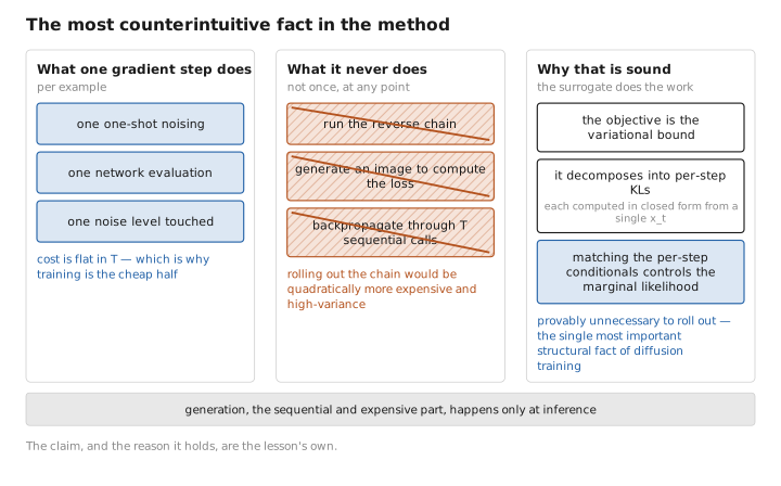
Figure 3. The most counterintuitive fact in the method.

Exercises

1. Unbiasedness of the loop. With $t\sim\mathcal U\{1,\dots,T\}$, show the single-draw loss $g=\|\epsilon-\epsilon_\theta(x_t,t)\|^2$ has expectation $\frac1T\sum_{t=1}^T\mathbb E_{x_0,\epsilon}\|\epsilon-\epsilon_\theta(x_t,t)\|^2$, so $\nabla_\theta g$ is an unbiased estimator of $\nabla_\theta L_\text{simple}$ up to the constant $1/T$.

Let $f(t)=\mathbb E_{x_0,\epsilon}\|\epsilon-\epsilon_\theta(x_t,t)\|^2$. Since $t$ is uniform, $\mathbb E_{t,x_0,\epsilon}[g]=\sum_{t=1}^T\frac1T f(t)=\frac1T\sum_t f(t)$. Gradients commute with the (finite) expectation: $\mathbb E[\nabla_\theta g]=\frac1T\sum_t\nabla_\theta f(t)=\frac1T\nabla_\theta\sum_t f(t)$. The factor $1/T$ is a fixed scalar absorbed into the learning rate, so the per-sample gradient is an unbiased estimator of $\nabla_\theta L_\text{simple}$ (which uses $\frac1T\sum_t$ via the uniform $t$).

2. Importance sampling stays unbiased. For any proposal $p(t)\gt 0$ and the estimator $\hat L=L_{t-1}/p(t)$, show $\mathbb E_{t\sim p}[\hat L]=\sum_t L_{t-1}$. What choice of $p(t)$ minimizes variance?

$\mathbb E_{t\sim p}[\hat L]=\sum_t p(t)\cdot\frac{L_{t-1}}{p(t)}=\sum_t L_{t-1}$ — unbiased for any $p(t)\gt 0$. Variance is reduced when $p(t)$ tracks the per-$t$ loss magnitude; for an unweighted sum the variance-minimizing proposal is $p(t)\propto\sqrt{\mathbb E[L_{t-1}^2]}$ (Nichol & Dhariwal maintain a running estimate of $\mathbb E[L_{t-1}^2]$).

3. Why data must be scaled to $[-1,1]$. If images are left in $[0,1]$ (so $\mathbb E[x_0]\approx0.5$, $\mathrm{Var}(x_0)\ne1$), what breaks at the terminal step, and why does it make $L_T$ non-negligible?

The forward marginal has mean $\sqrt{\bar\alpha_t}\,\mathbb E[x_0]$ and variance $\bar\alpha_t\mathrm{Var}(x_0)+(1-\bar\alpha_t)$. The variance-preserving design relies on $\mathrm{Var}(x_0)\approx1$ to keep this $\approx1$ for all $t$. With un-centered, un-scaled data the terminal $q(x_T)$ no longer matches the standard-normal prior $p(x_T)=\mathcal N(0,I)$, so $L_T=D_{\mathrm{KL}}(q(x_T\mid x_0)\,\|\,\mathcal N(0,I))$ becomes non-negligible and there is a train/sample prior mismatch (sampling starts from $\mathcal N(0,I)$, which the chain was not trained to land on). Centering and scaling to $[-1,1]$ restores the match.

4. EMA ordering. Why must ema.update(model) run after optimizer.step(), and what are the EMA weights used for?

EMA maintains a running average of the post-update parameters: $s\leftarrow d\,s+(1-d)\,\theta_{\text{new}}$. Calling it before the optimizer step would average stale, pre-update weights and lag the shadow by a step. The EMA shadow is used at sampling time (not for the gradient step) because the averaged weights give noticeably smoother, higher-quality samples.

Conclusion

Training is a five-line loop that is best understood as a doubly-stochastic Monte-Carlo estimator of $\sum_t L_{t-1}$: sample data, sample a timestep (uniform, importance-sampled, or Min-SNR-weighted), sample noise, jump to that noise level in one shot, and regress the network’s prediction onto the true target with MSE. The estimator is unbiased; its variance is controlled by batch size and by the timestep proposal. Practical convergence to a competitive model requires EMA weights, a cosine schedule, AdamW with warmup and gradient clipping, mixed precision, and consistent $[-1,1]$ data scaling — and optionally a $v$-prediction target when the SNR endpoints matter. None of this ever rolls out the reverse process. With $\epsilon_\theta$ (or $v_\theta$) trained, Lesson 8 finally runs the reverse chain: the DDPM sampling algorithm that turns pure noise into a sample.

The index card is written, and what it never does — run the reverse chain even once — is precisely the thing Lesson 8 does for the first time. We have a trained noise predictor; now we make it dream.

References

• J. Ho, A. Jain, P. Abbeel. Denoising Diffusion Probabilistic Models. NeurIPS 2020.
• A. Nichol, P. Dhariwal. Improved Denoising Diffusion Probabilistic Models. ICML 2021. (Cosine schedule; importance sampling over $t$; learned variances.)
• T. Salimans, J. Ho. Progressive Distillation for Fast Sampling of Diffusion Models. ICLR 2022. ($v$-prediction.)
• T. Karras, M. Aittala, T. Aila, S. Laine. Elucidating the Design Space of Diffusion-Based Generative Models (EDM). NeurIPS 2022. (Loss weighting and noise-level sampling.)
• T. Hang et al. Efficient Diffusion Training via Min-SNR Weighting Strategy. ICCV 2023.
• D. Kingma, T. Salimans, B. Poole, J. Ho. Variational Diffusion Models. NeurIPS 2021. (SNR-based formulation of the bound.)

← Previous: Lesson 6 — The U-Net Architecture · Course Index · Next: Lesson 8 — DDPM Sampling → · Appendix A: Acronyms · Appendix B: Formulas

The figures in this lesson follow the shared figure key , which explains what every shape, line style and colour means.