Lesson 8 — The Sampling Algorithm: Inference with DDPM

Recap of Lesson 7. Training is a five-line loop: sample $x_0$, sample $t\sim\mathcal U\{1,T\}$, sample $\epsilon\sim\mathcal N(0,I)$, form $x_t=\sqrt{\bar\alpha_t}x_0+\sqrt{1-\bar\alpha_t}\epsilon$ in one shot, and minimize $\|\epsilon-\epsilon_\theta(x_t,t)\|^2$. Crucially, training never runs the reverse chain; it uses the variational surrogate. EMA weights and a good schedule make it stable. Now we finally run the reverse chain to generate.

Until now the reverse process has been a thing we reasoned about but never ran. This lesson finally turns the crank. We begin with a square of pure static — no image, nothing, just a draw from a Gaussian — and put the same patient question to the trained network a thousand times over: what is the noise here, and what lies one notch beneath it? Slowly, out of the static, a face that never existed sharpens into view. The price of that thousand-fold patience is the very problem the next lesson exists to solve.

Overview

We have a trained noise predictor $\epsilon_\theta$ (use the EMA weights from Lesson 7). Generation inverts the forward corruption: initialize a canvas $x_T\sim\mathcal N(0,I)$ — matching the prior the forward process converges to — and iterate the learned reverse kernel down to $x_0$. Each step estimates the noise in the current state, removes a calibrated fraction of it, and re-injects a controlled amount of fresh randomness so that we draw from the conditional distribution rather than collapsing to its mode. After $T$ steps a coherent sample emerges. Unlike training, inference is inherently sequential, and that sequentiality is the central efficiency problem this lesson sets up.

The DDPM sampling step

We sample from the learned reverse Gaussian $p_\theta(x_{t-1}\mid x_t)=\mathcal N\!\big(\mu_\theta(x_t,t),\sigma_t^2 I\big)$. Using the $\epsilon$-parameterized mean from Lesson 5, the update is:

with $z = 0$ at the final step $t=1$ (we output the mean). Two standard variance choices work comparably well:

Derivation of the mean

The tractable forward posterior (Lesson 3) is Gaussian,

The training objective drives $p_\theta$ to match $q(x_{t-1}\mid x_t,x_0)$, so we set $\mu_\theta = \tilde\mu_t$ but with the unknown $x_0$ replaced by the estimate the network implies. Inverting the forward jump $x_t=\sqrt{\bar\alpha_t}x_0+\sqrt{1-\bar\alpha_t}\epsilon$ gives

Substituting $\hat x_0$ into $\tilde\mu_t$ and simplifying with $\alpha_t=1-\beta_t$ and $\bar\alpha_t=\alpha_t\bar\alpha_{t-1}$ collapses the two terms into the single $\epsilon$-form

which is the deterministic part of the boxed update. The reduction is purely algebraic; the cross-terms in $x_t$ cancel because $\sqrt{\alpha_t}(1-\bar\alpha_{t-1}) + \beta_t/\sqrt{\alpha_t}\cdot\bar\alpha_{t-1}\cdots$ regroup to $1/\sqrt{\alpha_t}$ times the bracket.

Why $\sigma_t^2\in\{\beta_t,\tilde\beta_t\}$

Remark (the two variances are bounds, Improved DDPM). With the mean fixed to $\tilde\mu_t$, the optimal reverse variance lies between two extremes. If the data were a single point ($x_0$ deterministic given $x_t$), the reverse conditional variance is exactly the posterior variance $\tilde\beta_t = \tfrac{1-\bar\alpha_{t-1}}{1-\bar\alpha_t}\beta_t$ (lower bound). If the data distribution is the standard normal, the reverse variance equals the forward variance $\beta_t$ (upper bound). One checks $\tilde\beta_t \le \beta_t$ for all $t$, with the gap small for most $t$ but large near $t=1$. Ho et al. (2020) found both endpoints give similar sample quality. Nichol & Dhariwal (2021) instead learn an interpolation in log-space,

$$\sigma_t^2 = \exp\!\big(v\log\beta_t + (1-v)\log\tilde\beta_t\big),\qquad v=v_\theta(x_t,t)\in[0,1],$$

trained with the full $\mathcal L_\text{vlb}$ (the simple loss is independent of the variance), which improves log-likelihood and enables high-quality sampling in far fewer steps.

Reading the update

• Deterministic denoising (the mean). $\mu_\theta$ removes the network’s noise estimate and rescales — it is the posterior mean $\tilde\mu_t$ with $\epsilon$ replaced by $\epsilon_\theta$, i.e. with $x_0$ replaced by $\hat x_0$.
• Stochastic injection. $\sigma_t z$ re-adds randomness because $p_\theta(x_{t-1}\mid x_t)$ is a distribution, not a point.

Remark (why re-inject noise). Taking the mean at every step would push the chain toward the mode of each conditional and, compounded over $T$ steps, toward an over-smoothed average image — a single high-probability blur rather than a sample. The forward process is genuinely stochastic; faithfully inverting it requires sampling $x_{t-1}\sim p_\theta(\cdot\mid x_t)$, which the $\sigma_t z$ term implements. The exception is the final step ($t=1$): there is no $x_0$ noise to model, so we emit the mean, $z=0$, avoiding an unnecessary variance injection on the output.

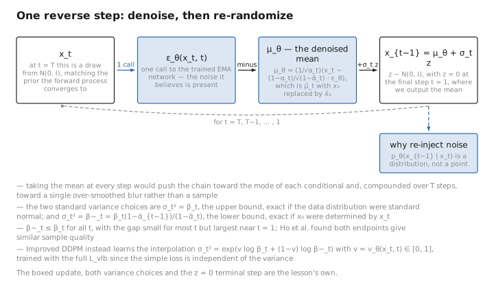
Figure 1. One reverse step: denoise, then re-randomize.

The full sampling algorithm (DDPM)

With the single step understood, the full procedure is simply that step, repeated with discipline from pure noise all the way down to a picture.

1. $x_T \sim \mathcal{N}(0, I)$    — start from pure noise
2. for $t = T, T-1, \dots, 1$ do
3.    $z \sim \mathcal{N}(0, I)$ if $t \gt 1$, else $z = 0$
4.    $x_{t-1} = \dfrac{1}{\sqrt{\alpha_t}}\left(x_t - \dfrac{1-\alpha_t}{\sqrt{1-\bar\alpha_t}}\,\epsilon_\theta(x_t, t)\right) + \sigma_t z$
5. end for
6. return $x_0$

Index convention (read once, then the code reads cleanly). The math indexes timesteps $t=1,\dots,T$; PyTorch arrays are 0-based, so the schedule buffers store level $t$ at position $t-1$. The loop variable i is the array position, and it runs downward T-1, …, 0. The single rule that resolves every cross-reference is:

$$ \texttt{i} \;=\; t-1 \qquad\Longleftrightarrow\qquad t \;=\; \texttt{i}+1. $$

loop i	math $t$	alpha_bars[i]	alpha_bars[i-1]	noise?
T-1	$T$	$\bar\alpha_T$	$\bar\alpha_{T-1}$	yes
…	…	…	…	yes
1	$2$	$\bar\alpha_2$	$\bar\alpha_1$	yes
0	$1$	$\bar\alpha_1$	$\bar\alpha_0:=1$ (guarded)	no ($z=0$)

So alpha_bars[i] is $\bar\alpha_t$ and alpha_bars[i-1] is $\bar\alpha_{t-1}$; the terminal iteration i=0 is the $t=1$ step that emits the mean. Whenever the code says [i], mentally read $\bar\alpha_t$; whenever it says [i-1], read $\bar\alpha_{t-1}$.

A complete, correct implementation supporting both $\sigma_t$ choices, optional $\hat x_0$ clamping / dynamic thresholding, and the $z=0$ terminal step:

@torch.no_grad()
def ddpm_sample(model, shape, diffusion, device,
                sigma_kind="tilde_beta",      # "beta" or "tilde_beta"
                thresholding="clamp",          # None | "clamp" | "dynamic"
                dynamic_p=0.995):
    """
    model:     trained EMA network, returns eps_theta(x_t, t), shape (B,C,H,W)
    diffusion: holds buffers betas, alphas, alpha_bars, all shape (T,)
    """
    betas, alphas, alpha_bars = diffusion.betas, diffusion.alphas, diffusion.alpha_bars
    T = diffusion.T
    x = torch.randn(shape, device=device)                       # x_T ~ N(0, I)

    for i in reversed(range(T)):                                # i = T-1, ..., 0  (=> t = i+1)
        t_batch = torch.full((shape[0],), i, device=device, dtype=torch.long)
        eps = model(x, t_batch)                                 # (B,C,H,W)

        a   = alphas[i]                                         # scalar tensors
        ab  = alpha_bars[i]
        b   = betas[i]
        ab_prev = alpha_bars[i - 1] if i > 0 else torch.ones((), device=device)

        # Predict x0, optionally constrain it (improves high-guidance stability).
        x0_hat = (x - (1 - ab).sqrt() * eps) / ab.sqrt()        # (B,C,H,W)
        if thresholding == "clamp":
            x0_hat = x0_hat.clamp(-1.0, 1.0)
        elif thresholding == "dynamic":                         # Imagen-style
            s = torch.quantile(x0_hat.abs().flatten(1), dynamic_p, dim=1)
            s = s.clamp(min=1.0).view(-1, 1, 1, 1)              # threshold >= 1
            x0_hat = x0_hat.clamp(-s, s) / s

        # Posterior mean tilde_mu_t(x_t, x0_hat); equivalent to the boxed eps-form.
        mean = (ab_prev.sqrt() * b / (1 - ab)) * x0_hat \
             + (a.sqrt() * (1 - ab_prev) / (1 - ab)) * x

        if i > 0:
            if sigma_kind == "beta":
                var = b
            else:                                               # tilde_beta (lower bound)
                var = (1 - ab_prev) / (1 - ab) * b
            x = mean + var.sqrt() * torch.randn_like(x)         # x_{t-1}
        else:
            x = mean                                            # t = 1: no noise injected
    return x                                                    # x_0, a fresh sample

Shape and correctness notes.

• Loop index i runs T-1 … 0, corresponding to timestep t = i+1; the terminal iteration i=0 is the $t=1$ step where $z=0$.
• alpha_bars[i-1] is undefined at i=0; we use $\bar\alpha_{-1}\equiv1$ there, but since that branch emits the mean only, the value is irrelevant — it is guarded so the deterministic-view code below is exact.
• Schedule buffers stay float32 to keep $\sqrt{1-\bar\alpha_t}$ stable for large $T$; cast x/eps as needed for AMP but reduce in float32.
• @torch.no_grad() is mandatory: no gradients are needed and it halves memory, allowing larger batches.

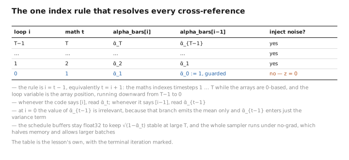
Figure 2. The one index rule that resolves every cross-reference.

An equivalent “predict $\hat x_0$, then re-noise” view

The code above already uses this view; here is why it equals the boxed update. At step $t$:

1. Estimate the clean image by inverting the forward jump: $$ \hat x_0 = \frac{1}{\sqrt{\bar\alpha_t}}\big(x_t - \sqrt{1-\bar\alpha_t}\,\epsilon_\theta(x_t,t)\big). $$
2. Re-noise to level $t-1$ by sampling $q(x_{t-1}\mid x_t,\hat x_0)=\mathcal N\!\big(\tilde\mu_t(x_t,\hat x_0),\tilde\beta_t I\big)$.

Proof of equivalence. Insert $\hat x_0$ into the posterior mean:

$$ \tilde\mu_t(x_t,\hat x_0) = \frac{\sqrt{\bar\alpha_{t-1}},\beta_t}{1-\bar\alpha_t},\hat x_0

• \frac{\sqrt{\alpha_t},(1-\bar\alpha_{t-1})}{1-\bar\alpha_t},x_t. $$

Substitute $\hat x_0 = \big(x_t-\sqrt{1-\bar\alpha_t}\,\epsilon_\theta\big)/\sqrt{\bar\alpha_t}$ and use $\bar\alpha_t=\alpha_t\bar\alpha_{t-1}$ so that $\sqrt{\bar\alpha_{t-1}}/\sqrt{\bar\alpha_t} = 1/\sqrt{\alpha_t}$. The coefficient of $x_t$ becomes

using $\beta_t+\alpha_t(1-\bar\alpha_{t-1}) = 1-\alpha_t+\alpha_t-\alpha_t\bar\alpha_{t-1} = 1-\bar\alpha_t$. The coefficient of $\epsilon_\theta$ is

Collecting the two coefficients yields exactly $\mu_\theta=\frac{1}{\sqrt{\alpha_t}}\big(x_t-\frac{1-\alpha_t}{\sqrt{1-\bar\alpha_t}}\epsilon_\theta\big)$, the deterministic part of the boxed update; with variance $\tilde\beta_t$ this is line 4 verbatim. $\;\blacksquare$

Conceptually: each step makes a full guess of the final image, then steps one notch back toward it. Early $\hat x_0$ is a blurry hallucination and sharpens as $t$ decreases.

Remark (clamping and dynamic thresholding). Because $\hat x_0$ is exposed explicitly, we can constrain it to the valid data range $[-1,1]$. Naive clamping helps at high classifier-free-guidance scales where the unconstrained $\hat x_0$ saturates. Saharia et al. (2022, Imagen) replace static clamping with dynamic thresholding: choose the per-image threshold $s$ as the $p$-th percentile of $|\hat x_0|$ (with $s\ge1$), clip to $[-s,s]$, then rescale by $1/s$. This prevents the oversaturation and color shifts that strong guidance otherwise causes, and is now standard in high-resolution text-to-image samplers (Lesson 10).

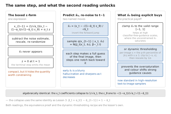
Figure 3. The same step, and what the second reading unlocks.

The cost of inference, and why it motivates Lesson 9

The sampler works — and in working, it hands us the bill that the rest of the course is devoted to paying down.

Remark (sequential cost and discretization error). Sampling calls the network once per step, and DDPM uses $T\approx1000$ steps, so one image needs ~1000 sequential forward passes — far slower than a GAN’s single pass. This is the practical weakness of diffusion. The deeper framing: the boxed update is the Euler–Maruyama discretization of a continuous-time reverse SDE, and $T$ is just the number of integration steps. The per-step error is a discretization error that vanishes as the step size shrinks; conversely, with a better integrator we can take far larger steps. Since $\epsilon_\theta$ was trained on a continuum of noise levels via the closed-form jump, inference is free to use a coarse, non-uniform subsequence of timesteps and even a deterministic ($\sigma_t=0$) update. That is exactly what DDIM exploits, and it opens the score-based / SDE view that unifies diffusion with stochastic calculus.

Exercises

1. Coefficient collapse. Substitute $\hat x_0=\frac{1}{\sqrt{\bar\alpha_t}}(x_t-\sqrt{1-\bar\alpha_t}\,\epsilon_\theta)$ into the posterior mean $\tilde\mu_t(x_t,\hat x_0)$ and show the coefficient of $x_t$ equals $1/\sqrt{\alpha_t}$.

Using $\sqrt{\bar\alpha_{t-1}}/\sqrt{\bar\alpha_t}=1/\sqrt{\alpha_t}$, the $x_t$-coefficient is

since $\beta_t+\alpha_t(1-\bar\alpha_{t-1})=1-\alpha_t+\alpha_t-\alpha_t\bar\alpha_{t-1}=1-\bar\alpha_t$.

2. The terminal step. Why do we set $z=0$ (emit the mean) at $t=1$ rather than injecting $\sigma_1 z$?

At the last step we sample $p_\theta(x_0\mid x_1)$ to produce the clean output; there is no further $x_0$-level noise to model, and the true posterior variance $\tilde\beta_1=0$. Emitting the mean avoids adding an unnecessary, quality-degrading variance injection to the final image.

3. Index sanity check. Using the index convention, at loop iteration i=0: what is the math timestep $t$, what value is used for $\bar\alpha_{t-1}$, and why is that value irrelevant to the output?

i=0 $\Rightarrow t=i+1=1$. Then $\bar\alpha_{t-1}=\bar\alpha_0:=1$ (the guarded value torch.ones(...)). It is irrelevant because at $t=1$ the code takes the no-noise branch and emits the mean ($z=0$); $\bar\alpha_{t-1}$ only ever enters the variance term, which is not used at this step.

4. The two variances. State the two standard choices of $\sigma_t^2$, say which is the lower and which the upper bound on the optimal reverse variance, and where the gap between them is largest.

$\sigma_t^2=\tilde\beta_t=\frac{1-\bar\alpha_{t-1}}{1-\bar\alpha_t}\beta_t$ is the lower bound (exact when the data is a single point given $x_t$); $\sigma_t^2=\beta_t$ is the upper bound (exact when the data is standard normal). One checks $\tilde\beta_t\le\beta_t$, with the gap small for most $t$ but largest near $t=1$. Ho et al. found both give comparable sample quality; Improved DDPM learns an interpolation between them.

Conclusion

Inference runs the learned reverse chain: start at $x_T\sim\mathcal N(0,I)$ and iterate the DDPM update, which subtracts the network’s predicted noise (the deterministic posterior mean $\mu_\theta=\tilde\mu_t$ with $x_0\to\hat x_0$) and re-injects $\sigma_t z$ — with $\sigma_t^2$ either $\beta_t$ (upper bound) or $\tilde\beta_t$ (lower bound), the two extremes that Improved DDPM interpolates by learning. The “predict $\hat x_0$, re-noise to $t-1$” view is algebraically identical to the boxed update and makes thresholding natural. The stochastic term is what samples from the distribution rather than its mode; the price is ~$T$ sequential network calls, a discretization of an underlying reverse SDE. In Lesson 9 we attack that cost with DDIM (fewer, deterministic steps) and reveal the deep score-based / SDE view.

We turned the crank and, a thousand steps later, a sample appeared. The obvious next question is whether we truly needed all thousand — and Lesson 9, in answering “no,” uncovers what the chain was all along: the clumsy discretization of a smooth, continuous flow.

References

• J. Ho, A. Jain, P. Abbeel. Denoising Diffusion Probabilistic Models. NeurIPS 2020. (Reverse update; $\sigma_t^2\in\{\beta_t,\tilde\beta_t\}$.)
• A. Nichol, P. Dhariwal. Improved Denoising Diffusion Probabilistic Models. ICML 2021. (Learned interpolated variance; few-step sampling.)
• J. Song, C. Meng, S. Ermon. Denoising Diffusion Implicit Models (DDIM). ICLR 2021. (Deterministic, accelerated sampling — Lesson 9.)
• C. Saharia et al. Photorealistic Text-to-Image Diffusion Models with Deep Language Understanding (Imagen). NeurIPS 2022. (Dynamic thresholding.)

← Previous: Lesson 7 — The Training Algorithm · Course Index · Next: Lesson 9 — DDIM & the Score View → · Appendix A: Acronyms · Appendix B: Formulas

The figures in this lesson follow the shared figure key , which explains what every shape, line style and colour means.