Lesson 9 — Faster & Deterministic Sampling (DDIM) and the Score View

Recap of Lesson 8. Inference runs the reverse chain: start at $x_T\sim\mathcal N(0,I)$ and iterate $x_{t-1}=\frac{1}{\sqrt{\alpha_t}}(x_t-\frac{1-\alpha_t}{\sqrt{1-\bar\alpha_t}}\epsilon_\theta) + \sigma_t z$ down to $x_0$. The deterministic part denoises; $\sigma_t z$ keeps samples diverse. An equivalent “predict $\hat x_0$, re-noise to $t{-}1$” view clarifies each step. The cost — ~$T=1000$ sequential network calls — is diffusion’s main weakness. We now make sampling fast and connect to score-based generative modeling.

A thousand sequential steps to make one picture is the kind of bill that limits what a method is allowed to become. This lesson is the escape, and it arrives in two acts. First the practical trick: the same trained network can descend the mountain in twenty strides instead of a thousand, and can be made to walk a single deterministic trail rather than a drunkard’s stagger. Then the deeper turn — the recognition that the trail was never a staircase at all but a smooth current, a differential equation, of which everything we have built is just one discretization among many.

Overview

DDPM’s slowness is structural: its reverse chain is Markov, so $x_{t-1}$ requires $x_t$ for all $T$ steps. The DDIM insight (Song et al., 2021a) is that the training objective $L_\text{simple}$ depends only on the marginals $q(x_t\mid x_0)$, not on the joint forward process. One can therefore construct an entire non-Markovian family of forward (and hence reverse) processes that all share those marginals — so the same trained $\epsilon_\theta$ is valid for every member. Members of this family permit (a) reverse updates that jump across arbitrary timestep subsequences and (b) a tunable injected-noise level $\sigma_t$ that can be sent to zero, making sampling deterministic.

A second, deeper lens identifies $\epsilon_\theta$ with a scaled estimate of the score $\nabla_{x_t}\log q_t(x_t)$. This recasts diffusion as the numerical solution of a stochastic differential equation, or of its deterministic probability-flow ODE — exposing the machinery of stochastic calculus and high-order ODE solvers that bring sampling to $\sim10$–$20$ steps. These two lenses are the same object viewed twice: deterministic DDIM is the first-order discretization of the probability-flow ODE.

Heads-up — a deliberate change in rigor. The DDIM half of this lesson (above) stays at the careful, fully-derived level of Lessons 2–5. The score / SDE half (below) is the one genuine difficulty spike in the course: it draws on stochastic calculus (Itô diffusions, Wiener processes, the Fokker–Planck equation) that we have not built up and will not. By design we therefore state the key results and sketch the intuition rather than prove them from first principles — the proofs live in the cited papers (Anderson 1982; Song et al. 2021b). You can read this section for the picture — “$\epsilon_\theta$ is a score; generation is integrating a reverse-time SDE or its ODE twin” — and lose nothing needed for Lesson 10 or for using the models. Treat the “Derivation (idea)” and “Proof sketch” boxes as motivation, not as the load-bearing inductive proofs of the earlier lessons.

DDIM: non-Markovian, optionally deterministic

The escape begins with a question that sounds almost like cheating: what if the chain we trained was never the only chain consistent with what the network actually learned?

The non-Markovian forward family

Fix the DDPM marginals $q(x_t\mid x_0)=\mathcal N(\sqrt{\bar\alpha_t}\,x_0,(1-\bar\alpha_t)I)$. Define a family indexed by a vector $\sigma=(\sigma_1,\dots,\sigma_T)$ of inference reverse-conditionals

The mean is engineered so that the family is marginal-preserving: by induction $q_\sigma(x_t\mid x_0)=\mathcal N(\sqrt{\bar\alpha_t}\,x_0,(1-\bar\alpha_t)I)$ for every choice of $\sigma$.

Derivation (marginal consistency). Assume $x_t=\sqrt{\bar\alpha_t}\,x_0+\sqrt{1-\bar\alpha_t}\,\epsilon$ with $\epsilon\sim\mathcal N(0,I)$. Substituting into the mean above, the data term contributes $\sqrt{\bar\alpha_{t-1}}\,x_0$ and the second term contributes $\sqrt{1-\bar\alpha_{t-1}-\sigma_t^2}\,\epsilon$. Adding the noise $\sigma_t z$ ($z\perp\epsilon$), the conditional variance of $x_{t-1}$ given $x_0$ is $(1-\bar\alpha_{t-1}-\sigma_t^2)+\sigma_t^2=1-\bar\alpha_{t-1}$, and the mean is $\sqrt{\bar\alpha_{t-1}}\,x_0$. Hence $x_{t-1}=\sqrt{\bar\alpha_{t-1}}\,x_0+\sqrt{1-\bar\alpha_{t-1}}\,\epsilon'$, $\epsilon'\sim\mathcal N(0,I)$ — exactly $q(x_{t-1}\mid x_0)$. The marginals are independent of $\sigma$. $\square$

Because the marginals match, the variational objective reduces (Song et al., 2021a, Thm. 1) to the same per-step denoising regression $L_\text{simple}$ used in Lesson 5. The trained $\epsilon_\theta$ is therefore reused unchanged across the whole family.

The DDIM reverse update

At sampling time $x_0$ is unknown; we substitute the model’s estimate $\hat x_0=(x_t-\sqrt{1-\bar\alpha_t}\,\epsilon_\theta(x_t,t))/\sqrt{\bar\alpha_t}$ (Tweedie/posterior-mean, below) into the conditional mean, giving:

Read it as three pieces: predict the clean image $\hat x_0$, scale it to level $t-1$, add a deterministic “direction” term built from the same predicted noise, and optionally add stochastic noise $\sigma_t z$.

Recovering the two extremes

• $\sigma_t=\sqrt{\tilde\beta_t}$ recovers DDPM. Setting the injected variance to the true posterior variance $\tilde\beta_t=\frac{1-\bar\alpha_{t-1}}{1-\bar\alpha_t}\beta_t$ makes $q_\sigma(x_{t-1}\mid x_t,x_0)$ coincide with the DDPM posterior $q(x_{t-1}\mid x_t,x_0)$ from Lesson 3, and the update reduces algebraically to the Lesson 8 sampler. The process becomes Markov again.
• $\sigma_t=0$ gives deterministic DDIM. All randomness vanishes after $x_T$; the map $x_T\mapsto x_0$ is a deterministic function. The update becomes $$ x_{t-1}=\sqrt{\bar\alpha_{t-1}}\,\hat x_0+\sqrt{1-\bar\alpha_{t-1}}\;\epsilon_\theta(x_t,t), $$ which we will recognize below as the first-order integrator of the probability-flow ODE.

Remark (interpolating regimes). A common parameterization is $\sigma_t=\eta\,\sqrt{\tilde\beta_t}$ with $\eta\in[0,1]$: $\eta=1$ is DDPM, $\eta=0$ is deterministic DDIM, and intermediate $\eta$ trades sample diversity against few-step fidelity. The choice is orthogonal to training.

Two big payoffs

1. Fewer steps. Because the update references $\bar\alpha$ at arbitrary levels, it runs on a subsequence $\tau_1\lt \dots\lt \tau_S$ of $\{1,\dots,T\}$ with $S\ll T$. Each accelerated step maps $x_{\tau_i}\to x_{\tau_{i-1}}$ using $\bar\alpha_{\tau_i},\bar\alpha_{\tau_{i-1}}$. With $\eta=0$, 20–50 steps often rival 1000 DDPM steps.
2. A meaningful latent space. Deterministic DDIM, being an ODE discretization, is approximately invertible: running the update forward (the DDIM inversion, $x_t\to x_{t+1}$ with the same $\epsilon_\theta$) recovers a near-unique $x_T$. This makes $x_T\leftrightarrow x_0$ a near-bijection, enabling semantic interpolation (slerp two $x_T$’s, decode, get a smooth morph) and real-image editing (invert a real image to $x_T$, edit, regenerate) — both impossible with stochastic DDPM.

Remark (inversion fidelity). DDIM inversion is exact only in the continuous limit; at finite step counts and with strong classifier-free guidance (Lesson 10) the local linearization error accumulates, and reconstruction drifts. Null-text inversion and exact-inversion solvers exist to mitigate this.

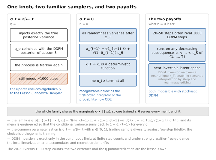
Figure 1. One knob, two familiar samplers, and two payoffs.

The score-based / SDE perspective

(This is the stated-results-and-intuition section flagged in the overview; stochastic-calculus background is assumed but not required to follow the picture.)

The unifying lens (Song & Ermon, 2019; Song et al., 2021b). Define the score of a distribution as the gradient of its log-density w.r.t. the input:

Tweedie’s formula and the score identity

Theorem (Tweedie’s formula; Robbins, Efron). Let $x_0\sim p$ and let $x_t=\sqrt{\bar\alpha_t}\,x_0+\sqrt{1-\bar\alpha_t}\,\epsilon$, $\epsilon\sim\mathcal N(0,I)$, so the noisy marginal is $q_t(x_t)=\int \mathcal N(x_t;\sqrt{\bar\alpha_t}x_0,(1-\bar\alpha_t)I)\,p(x_0)\,dx_0$. Then the posterior mean of the clean scaled signal satisfies

$$ \gt \mathbb E[\sqrt{\bar\alpha_t}\,x_0\mid x_t]=x_t+(1-\bar\alpha_t)\,\nabla_{x_t}\log q_t(x_t). \gt $$

Proof sketch. For the Gaussian likelihood $q_t(x_t\mid x_0)=\mathcal N(\sqrt{\bar\alpha_t}x_0,(1-\bar\alpha_t)I)$, differentiate under the integral: $\nabla_{x_t}q_t(x_t)=\int \frac{\sqrt{\bar\alpha_t}x_0-x_t}{1-\bar\alpha_t}\,q_t(x_t\mid x_0)p(x_0)\,dx_0$. Dividing by $q_t(x_t)$ gives $\nabla_{x_t}\log q_t(x_t)=\frac{1}{1-\bar\alpha_t}\big(\mathbb E[\sqrt{\bar\alpha_t}x_0\mid x_t]-x_t\big)$. Rearranging yields the stated formula. $\square$

Now connect to the noise. Since $x_t=\sqrt{\bar\alpha_t}x_0+\sqrt{1-\bar\alpha_t}\,\epsilon$, the posterior mean of $\sqrt{\bar\alpha_t}x_0$ equals $x_t-\sqrt{1-\bar\alpha_t}\,\mathbb E[\epsilon\mid x_t]$. Substituting into Tweedie:

The denoising-score-matching optimum is $\epsilon_\theta(x_t,t)=\mathbb E[\epsilon\mid x_t]$ (the MSE-minimizer is the conditional mean), so:

So training $\epsilon_\theta$ to predict noise is, up to the known scaling $-1/\sqrt{1-\bar\alpha_t}$, training a model of the score at every noise level. The simple loss of Lesson 5 is weighted denoising score matching in disguise. Equivalently, the posterior-mean estimate $\hat x_0$ used in the DDIM update is the Tweedie estimator.

With a score model one can also generate by annealed Langevin dynamics — stepping along the score plus noise:

a stochastic walk toward high-density regions; this is the original NCSN sampler (Song & Ermon, 2019).

Continuous time: the VP-SDE

Take $T\to\infty$ so the discrete chain becomes a continuous-time stochastic differential equation (SDE). The DDPM discretization corresponds to the variance-preserving (VP) SDE (Song et al., 2021b). Writing $\beta(t)$ for the continuous-time noise rate,

with $w$ a standard Wiener process; here $f(x,t)=-\tfrac12\beta(t)x$ and $g(t)=\sqrt{\beta(t)}$. Its transition kernel is Gaussian with mean-scale $\exp(-\tfrac12\int_0^t\beta(s)ds)$ and matches the discrete $\bar\alpha_t$ in the limit, recovering $q_t(x_t\mid x_0)=\mathcal N(\sqrt{\bar\alpha_t}x_0,(1-\bar\alpha_t)I)$.

Theorem (Anderson, 1982; reverse-time SDE). A diffusion $dx=f(x,t)dt+g(t)dw$ run forward from $t=0$ to $T$ admits a time-reversal that is itself a diffusion:

$$ \gt dx=\big[f(x,t)-g(t)^2\,\nabla_x\log q_t(x)\big]dt+g(t)\,d\bar w, \gt $$

where $\bar w$ is a Wiener process in reverse time and $q_t$ is the forward marginal at time $t$. The reverse drift depends on the data only through the score $\nabla_x\log q_t$.

Substituting the learned score $-\epsilon_\theta/\sqrt{1-\bar\alpha_t}$ and integrating this reverse SDE from $t=T$ to $0$ is generation. The DDPM ancestral sampler of Lesson 8 is the Euler–Maruyama discretization of the VP reverse SDE.

The probability-flow ODE — the fast lane

Every diffusion SDE has an associated deterministic probability-flow ODE whose trajectories have the same marginal densities $q_t$ at every time (Song et al., 2021b, Prop. 1, via the Fokker–Planck equation):

Derivation (idea). The forward Fokker–Planck equation $\partial_t q_t=-\nabla\!\cdot(f q_t)+\tfrac12 g^2\nabla^2 q_t$ can be rewritten as a continuity equation $\partial_t q_t=-\nabla\!\cdot(\tilde f q_t)$ with effective drift $\tilde f=f-\tfrac12 g^2\nabla\log q_t$ and no diffusion term. Any deterministic flow with velocity $\tilde f$ transports the same density family, hence shares the marginals. $\square$

Because it is an ODE, one can apply mature numerical integrators — Heun/RK methods, DEIS, and DPM-Solver (Lu et al., 2022) exploit the semilinear structure (the exact solution of the linear part plus a learned-term integral) to reach high quality in as few as 10–20 steps. The EDM framework (Karras et al., 2022) further clarifies preconditioning, noise schedules, and second-order correction.

Remark (DDIM = first-order ODE discretization). Substituting the score identity into the VP probability-flow ODE and integrating one step with the exponential-integrator (change of variables to $\lambda_t=\log(\sqrt{\bar\alpha_t}/\sqrt{1-\bar\alpha_t})$, the log-SNR) yields exactly the deterministic ($\sigma_t=0$) DDIM update. DDIM is therefore the first-order member of the DPM-Solver family, and higher-order solvers are its principled generalization.

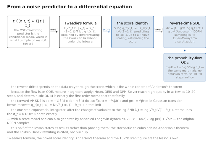
Figure 2. From a noise predictor to a differential equation.

Predicting $v$ instead of $\epsilon$

One practical footnote before we leave the chapter — the regression target that quietly powers most fast and high-resolution models.

A practical reparameterization used in fast/distilled and high-resolution models: predict $v := \sqrt{\bar\alpha_t}\,\epsilon - \sqrt{1-\bar\alpha_t}\,x_0$ (Salimans & Ho, 2022). The $v$-parameterization keeps the regression target well-scaled across all noise levels — at $t\to T$ where $\epsilon$-prediction is fine but $x_0$-prediction degenerates, and at $t\to 0$ where the reverse holds — and is the natural target on the velocity field of the probability-flow ODE. It improves stability at high resolution and is the standard target for progressive distillation, which halves the step count repeatedly to compress 1000 steps into a handful.

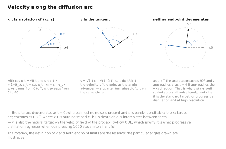
Figure 3. Velocity along the diffusion arc.

Code: a DDIM sampler

import torch

@torch.no_grad()
def ddim_sample(model, shape, alphabar, timesteps, eta=0.0, device="cuda"):
    """
    model:      eps_theta(x_t, t) -> noise estimate, same shape as x_t
    shape:      (B, C, H, W)
    alphabar:   tensor of cumulative products bar_alpha_t, indexed by global t in [0, T-1]
    timesteps:  decreasing subsequence of ints, e.g. list(range(999, -1, -20))
    eta:        0.0 -> deterministic DDIM; 1.0 -> DDPM-equivalent stochasticity
    returns:    x_0 estimate, shape == shape
    """
    x = torch.randn(shape, device=device)                      # x_T ~ N(0, I), (B,C,H,W)
    for i, t in enumerate(timesteps):
        t_next = timesteps[i + 1] if i + 1 < len(timesteps) else -1
        ab_t      = alphabar[t]                                 # scalar bar_alpha_t
        ab_prev   = alphabar[t_next] if t_next >= 0 else torch.tensor(1.0, device=device)

        t_batch = torch.full((shape[0],), t, device=device, dtype=torch.long)  # (B,)
        eps     = model(x, t_batch)                             # (B,C,H,W)

        # Tweedie / predicted clean image  hat_x0  (B,C,H,W)
        x0_pred = (x - (1 - ab_t).sqrt() * eps) / ab_t.sqrt()
        x0_pred = x0_pred.clamp(-1, 1)                          # optional stabilization

        # sigma_t = eta * sqrt(tilde_beta_t);  tilde_beta_t = (1-ab_prev)/(1-ab_t) * (1 - ab_t/ab_prev)
        sigma = eta * (((1 - ab_prev) / (1 - ab_t)) * (1 - ab_t / ab_prev)).clamp(min=0).sqrt()

        # direction term uses the SAME eps; (1 - ab_prev - sigma^2) >= 0 by construction
        dir_xt = (1 - ab_prev - sigma**2).clamp(min=0).sqrt() * eps
        noise  = sigma * torch.randn_like(x) if eta > 0 else 0.0

        x = ab_prev.sqrt() * x0_pred + dir_xt + noise          # x_{t_next}, (B,C,H,W)
    return x

Numerical notes. (i) alphabar indexing must use the global timestep, not the loop index, so accelerated subsequences read the correct $\bar\alpha$. (ii) Clamping $\hat x_0$ to the data range stabilizes few-step sampling and is the simple precursor of dynamic thresholding (Lesson 10). (iii) The clamp(min=0) guards against tiny negative radicands from float error near $t\approx T$. (iv) For classifier-free guidance, replace eps with the guided estimate before computing x0_pred (Lesson 10). (v) Use float32 for alphabar; accumulating $\bar\alpha_t$ in float16 loses precision at small $\beta_t$.

Exercises

1. Marginal consistency. In the DDIM family, with $x_t=\sqrt{\bar\alpha_t}\,x_0+\sqrt{1-\bar\alpha_t}\,\epsilon$, show that the conditional variance of $x_{t-1}$ given $x_0$ equals $1-\bar\alpha_{t-1}$ (so the marginal matches $q(x_{t-1}\mid x_0)$ for any $\sigma_t$).

The mean’s “direction” term contributes $\sqrt{1-\bar\alpha_{t-1}-\sigma_t^2}\,\epsilon$ (variance $1-\bar\alpha_{t-1}-\sigma_t^2$) and the added stochastic term contributes $\sigma_t z$ with $z\perp\epsilon$ (variance $\sigma_t^2$). Being independent, the variances add: $(1-\bar\alpha_{t-1}-\sigma_t^2)+\sigma_t^2=1-\bar\alpha_{t-1}$. The mean is $\sqrt{\bar\alpha_{t-1}}\,x_0$, so $x_{t-1}\sim\mathcal N(\sqrt{\bar\alpha_{t-1}}x_0,(1-\bar\alpha_{t-1})I)=q(x_{t-1}\mid x_0)$, independent of $\sigma_t$.

2. Recovering the two extremes. Show that $\sigma_t=0$ gives the deterministic DDIM update, and explain why $\sigma_t=\sqrt{\tilde\beta_t}$ makes the process Markov again (DDPM).

Setting $\sigma_t=0$ drops the $\sigma_t z$ term and makes $\sqrt{1-\bar\alpha_{t-1}-\sigma_t^2}=\sqrt{1-\bar\alpha_{t-1}}$, leaving $x_{t-1}=\sqrt{\bar\alpha_{t-1}}\,\hat x_0+\sqrt{1-\bar\alpha_{t-1}}\,\epsilon_\theta$ — a deterministic map. Setting $\sigma_t=\sqrt{\tilde\beta_t}$ injects exactly the true posterior variance of Lesson 3, so $q_\sigma(x_{t-1}\mid x_t,x_0)$ coincides with the DDPM posterior $q(x_{t-1}\mid x_t,x_0)$ and the update reduces to the Lesson 8 ancestral sampler — the chain is Markov again.

3. The score–noise identity. Combine Tweedie’s formula $\mathbb E[\sqrt{\bar\alpha_t}x_0\mid x_t]=x_t+(1-\bar\alpha_t)\nabla_{x_t}\log q_t(x_t)$ with $\sqrt{\bar\alpha_t}x_0=x_t-\sqrt{1-\bar\alpha_t}\,\epsilon$ to derive $\nabla_{x_t}\log q_t(x_t)=-\mathbb E[\epsilon\mid x_t]/\sqrt{1-\bar\alpha_t}$, and hence the $\epsilon_\theta\leftrightarrow$ score relation.

Taking conditional expectations, $\mathbb E[\sqrt{\bar\alpha_t}x_0\mid x_t]=x_t-\sqrt{1-\bar\alpha_t}\,\mathbb E[\epsilon\mid x_t]$. Equating with Tweedie:

Since the MSE-optimal predictor is the conditional mean, $\epsilon_\theta(x_t,t)\approx\mathbb E[\epsilon\mid x_t]$, giving $\nabla_{x_t}\log q_t(x_t)\approx-\epsilon_\theta(x_t,t)/\sqrt{1-\bar\alpha_t}$: predicting noise is (scaled) score estimation.

4. DDIM as a first-order solver (conceptual). In one or two sentences, explain in what precise sense deterministic DDIM is the first-order discretization of the probability-flow ODE.

Substituting the score identity into the VP probability-flow ODE and integrating one step with an exponential integrator (changing variables to the log-SNR $\lambda_t=\log(\sqrt{\bar\alpha_t}/\sqrt{1-\bar\alpha_t})$) reproduces exactly the $\sigma_t=0$ DDIM update. DDIM is thus the first-order member of the DPM-Solver family; higher-order solvers (Heun, DPM-Solver-2/3) are principled generalizations that take larger, more accurate steps.

Conclusion

DDIM arises from a non-Markovian forward family with marginals matched to $q(x_t\mid x_0)$, so the trained $\epsilon_\theta$ transfers unchanged; choosing $\sigma_t=\sqrt{\tilde\beta_t}$ recovers DDPM and $\sigma_t=0$ gives a deterministic, timestep-skipping map (20–50 steps rivaling 1000) with a near-invertible latent space for interpolation and editing. The score view, grounded in Tweedie’s formula, shows $\epsilon_\theta$ is a scaled estimate of $\nabla_{x_t}\log q_t(x_t)$, recasting generation as integrating Anderson’s reverse-time SDE — or its marginal-equivalent probability-flow ODE, which Heun/DEIS/DPM-Solver crack in $\sim10$–$20$ steps, with deterministic DDIM as the first-order case. The $v$-parameterization keeps targets well-scaled for distillation and high resolution. We can now train and sample efficiently. Lesson 10 adds the final, practical layer: conditioning and guidance (steering generation with text or labels) and latent diffusion (how Stable Diffusion makes it all affordable).

Fast to train, fast to sample, and revealed as the discretization of a continuous flow — the chain has given up its last secret. Only one capability is still missing: the ability to ask for what we want. Lesson 10 supplies it, and with it the modern text-to-image stack.

References

• J. Song, C. Meng, S. Ermon. Denoising Diffusion Implicit Models (DDIM). ICLR 2021a.
• Y. Song, S. Ermon. Generative Modeling by Estimating Gradients of the Data Distribution (NCSN). NeurIPS 2019.
• Y. Song, J. Sohl-Dickstein, D. P. Kingma, A. Kumar, S. Ermon, B. Poole. Score-Based Generative Modeling through Stochastic Differential Equations. ICLR 2021b.
• B. D. O. Anderson. Reverse-time diffusion equation models. Stochastic Processes and their Applications, 1982.
• B. Efron. Tweedie’s Formula and Selection Bias. JASA 2011 (after H. Robbins, 1956).
• C. Lu, Y. Zhou, F. Bao, J. Chen, C. Li, J. Zhu. DPM-Solver. NeurIPS 2022.
• T. Karras, M. Aittala, T. Aila, S. Laine. Elucidating the Design Space of Diffusion-Based Generative Models (EDM). NeurIPS 2022.
• T. Salimans, J. Ho. Progressive Distillation for Fast Sampling of Diffusion Models ($v$-prediction). ICLR 2022.

← Previous: Lesson 8 — DDPM Sampling · Course Index · Next: Lesson 10 — Conditioning & Guidance → · Appendix A: Acronyms · Appendix B: Formulas

The figures in this lesson follow the shared figure key , which explains what every shape, line style and colour means.