Lesson 10 — Conditioning, Guidance, and the Modern Landscape
Recap of Lesson 9. DDIM rewrites the reverse step as “predict $\hat x_0$ + direction term + optional $\sigma_t z$”; with $\sigma_t=0$ it is deterministic, lets us skip timesteps (20–50 ≈ 1000), and gives an invertible latent space. The score view shows $\epsilon_\theta \approx -\sqrt{1-\bar\alpha_t}\,\nabla_x\log q_t(x)$, recasting generation as solving a reverse-time SDE or its probability-flow ODE (fast ODE solvers → ~10–20 steps). The $v$-parameterization keeps targets well-scaled. This final lesson adds steering and scale.
The model we have trained is a gifted sleepwalker. Left to itself it produces faces, landscapes, rooms — all plausible, none of them requested. It has no notion of “a red bicycle at dusk” and no reason to acquire one. This final lesson is about teaching it to take instruction: how to feed a prompt into the machine, why a naively conditioned model only half-listens, and the surprisingly sharp trick — guidance — that makes it obey. Then, because obedience at full resolution is ruinously expensive, how the entire performance is quietly moved into a smaller room.
Overview
So far we sample from the data distribution unconditionally — we cannot ask for “a photo of a red bicycle at dusk.” Real systems are conditional: given a prompt $c$ (text, class label, image) they sample from $p_\theta(x_0\mid c)$. Two ideas define the modern era. Guidance makes conditioning actually bite: naive conditioning under-weights $c$, and guidance amplifies it by reshaping the sampled distribution toward $p(x)p(c\mid x)^w$. Latent diffusion runs the entire process in a compressed autoencoder space, slashing cost. Together they are the recipe behind Stable Diffusion and its descendants. We close with a rigorous orientation on the contemporary stack — DiT, distillation, and flow matching.
Conditional diffusion
The framework barely changes: feed $c$ into the network, $\epsilon_\theta(x_t,t,c)$, and train on paired data with the same loss
$$ L = \mathbb{E}_{t,x_0,\epsilon,c}\big[\|\epsilon - \epsilon_\theta(x_t, t, c)\|^2\big]. $$By the same Tweedie/score argument of Lesson 9, the minimizer satisfies the conditional score identity
$$ \epsilon_\theta(x_t,t,c) \approx -\sqrt{1-\bar\alpha_t}\,\nabla_{x_t}\log q_t(x_t\mid c). $$For text, $c$ is an embedding from a frozen text encoder (CLIP or T5) injected via cross-attention (detailed below). The problem: a network trained this way tends to under-use $c$, producing samples that only loosely respect the prompt — the conditional density is “too flat.” The fix is guidance.
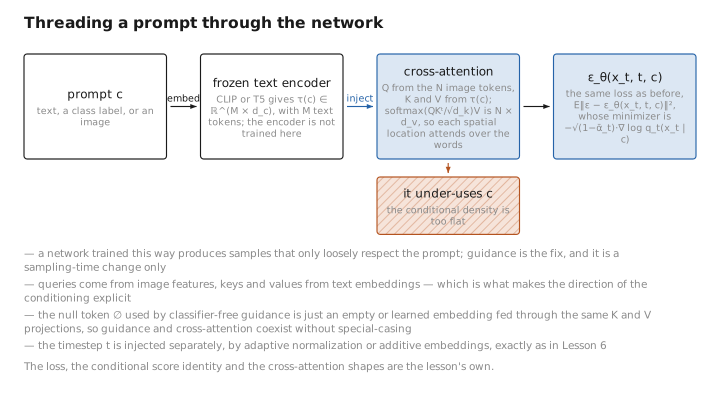
Figure 1. Threading a prompt through the network.
Classifier guidance
The first fix for an inattentive model came from outside the network entirely: borrow a critic who already knows the categories, and let it tug each sample into line.
The first approach (Dhariwal & Nichol, 2021) decomposes the conditional score by Bayes’ rule. From $\log q_t(x_t\mid c)=\log q_t(x_t)+\log p(c\mid x_t)-\log p(c)$, take $\nabla_{x_t}$ (the $\log p(c)$ term vanishes):
$$ \nabla_{x_t}\log q_t(x_t\mid c) = \nabla_{x_t}\log q_t(x_t) + \nabla_{x_t}\log p(c\mid x_t). $$Tilting the distribution by a power $w$
To amplify the condition, scale the classifier term by a guidance weight $w$, targeting the score of the tilted distribution $\tilde p_w(x_t\mid c)\propto q_t(x_t)\,p(c\mid x_t)^w$:
$$ \nabla_{x_t}\log \tilde p_w(x_t\mid c) = \nabla_{x_t}\log q_t(x_t) + w\,\nabla_{x_t}\log p(c\mid x_t). $$Derivation (implied distribution). The tilt $p(c\mid x)^w$ raises the likelihood to a power: for $w\gt 1$ it sharpens the posterior, concentrating mass where the classifier is confident (lower entropy, higher fidelity, less diversity); $w=1$ is the true posterior; $w\lt 1$ flattens it. The marginal over $c$ is $p_w(x)\propto p(x)\,\mathbb E_{c}[\,\cdots]$, but per-condition the operative target is $p(x)\,p(c\mid x)^w$.
Converting scores to noise via $\epsilon=-\sqrt{1-\bar\alpha_t}\,\nabla_{x_t}\log(\cdot)$ gives the guided noise estimate:
$$ \boxed{\ \hat\epsilon = \epsilon_\theta(x_t,t) - w\,\sqrt{1-\bar\alpha_t}\;\nabla_{x_t}\log p_\phi(c\mid x_t)\ } $$Larger $w$ → stronger adherence to $c$ at the cost of diversity. The drawback: one must train and run a noise-robust classifier $p_\phi(c\mid x_t)$ at every noise level — extra machinery, and its gradients can be adversarially brittle.
Classifier-free guidance (CFG) — the standard today
The elegant alternative (Ho & Salimans, 2022) needs no separate classifier. During training, randomly drop the condition (replace $c$ with a null token $\varnothing$) some fraction of the time (e.g. 10–20%). The same network thereby learns both the conditional $\epsilon_\theta(x_t,t,c)$ and the unconditional $\epsilon_\theta(x_t,t,\varnothing)$.
Deriving CFG from the score identity
Apply the score identity to both. By Bayes’ rule, the implicit classifier gradient is
$$ \nabla_{x_t}\log p(c\mid x_t)=\nabla_{x_t}\log q_t(x_t\mid c)-\nabla_{x_t}\log q_t(x_t) \approx -\frac{1}{\sqrt{1-\bar\alpha_t}}\big(\epsilon_\theta(x_t,t,c)-\epsilon_\theta(x_t,t,\varnothing)\big). $$Substitute this into the classifier-guidance target $\nabla\log q_t(x_t)+w\,\nabla\log p(c\mid x_t)$ and convert back to noise:
$$ \boxed{\ \hat\epsilon(x_t,t,c) = \epsilon_\theta(x_t,t,\varnothing) + w\,\big(\epsilon_\theta(x_t,t,c) - \epsilon_\theta(x_t,t,\varnothing)\big)\ } $$So CFG approximately samples from $p(x)\,p(c\mid x)^w$ using the model’s own conditional/unconditional difference as a built-in classifier gradient — no auxiliary network.
- $w = 1$: ordinary conditional sampling.
- $w \gt 1$ (typically 3–15): extrapolate past the conditional, away from the unconditional — strongly amplifying prompt adherence. This is the “guidance scale” / “CFG scale” knob in tools like Stable Diffusion.
It costs two network evaluations per step (the conditional and unconditional passes can be batched).
Remark (over-saturation and dynamic thresholding). High $w$ pushes $\hat x_0$ outside the valid data range $[-1,1]$, producing over-saturated, blown-out images. Dynamic thresholding (Saharia et al., 2022, Imagen) rescales each predicted $\hat x_0$ by a per-step percentile $s=\mathrm{percentile}(|\hat x_0|, p)$ (e.g. $p=99.5\%$): clip to $[-s,s]$ then divide by $\max(s,1)$. This pushes saturated pixels inward and preserves detail, enabling much larger $w$ than static clamping. The CFG weight, the schedule, and thresholding are all sampling-time choices, orthogonal to training.
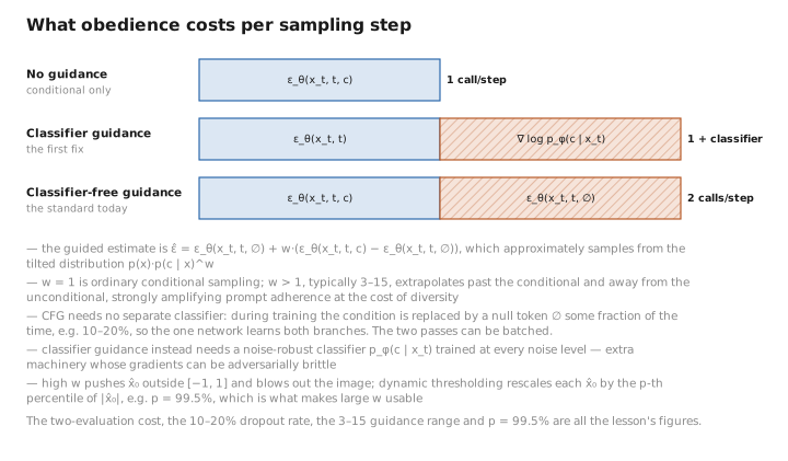
Figure 2. What obedience costs per sampling step.
Cross-attention conditioning
Text conditioning is implemented by cross-attention layers interleaved with the backbone’s self-attention (Rombach et al., 2022). Let $\phi(x_t)\in\mathbb R^{N\times d}$ be flattened image/latent features ($N$ spatial tokens) and $\tau(c)\in\mathbb R^{M\times d_c}$ the text token embeddings ($M$ tokens). Then
$$ Q=\phi(x_t)W_Q\;(N\times d_k),\quad K=\tau(c)W_K\;(M\times d_k),\quad V=\tau(c)W_V\;(M\times d_v), $$$$ \text{Attention}=\mathrm{softmax}\!\Big(\tfrac{QK^\top}{\sqrt{d_k}}\Big)V\;\in\mathbb R^{N\times d_v}. $$Queries come from image features; keys and values come from text embeddings. Each spatial location thus attends over the text tokens and pulls in the embeddings of the words relevant to it. The null token $\varnothing$ for CFG is just an empty/learned embedding fed through the same $K,V$ projections, so CFG and cross-attention coexist seamlessly. Time $t$ is injected separately (adaptive normalization / additive embeddings), as in Lesson 6.
Latent diffusion — making it affordable
Steering solved, one obstacle still stands between us and a usable system: raw pixels are simply too expensive to denoise a thousand times over.
Diffusion on raw $512\times512\times3$ pixels is enormously costly. Latent Diffusion Models (LDM) (Rombach et al., 2022 — the Stable Diffusion architecture) move the whole process into a compressed space:
- Pretrain an autoencoder. An encoder $E$ maps an image to a small latent $z_0=E(x)$ (e.g. $512\times512\times3 \to 64\times64\times4$, an $8\times$ spatial / $\sim48\times$ overall compression factor), and a decoder reconstructs $x\approx D(z_0)$. It is trained with a perceptual (LPIPS) + patch-adversarial loss for sharp reconstructions, plus a latent regularizer: either a small KL penalty toward $\mathcal N(0,I)$ (KL-VAE, continuous latents) or a VQ codebook (discrete latents). The regularizer keeps the latent space well-scaled so diffusion is well-conditioned.
- Run diffusion in latent space. Apply everything from Lessons 2–9 to $z_0$ instead of $x_0$: forward noising on $z$, train $\epsilon_\theta(z_t,t,c)$, sample with DDIM/ODE solvers and CFG. Cross-attention and CFG live entirely inside this latent-space backbone.
- Decode once. Map the generated latent back to pixels with $D(z_0)$ — a single forward pass, not part of the diffusion loop.
Because the latent grid is $\sim64\times$ smaller in element count, training and sampling are vastly cheaper — this is what put high-quality text-to-image generation on consumer GPUs.
Remark (separation of concerns). The autoencoder is frozen during diffusion training. Reconstruction fidelity is upper-bounded by $D(E(x))$; the diffusion model only ever sees the latent manifold, so artifacts can originate either in the latent prior (diffusion) or the decoder.
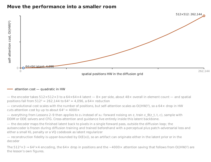
Figure 3. Move the performance into a smaller room.
The contemporary picture (rigorous orientation, not exhaustive)
- Diffusion Transformers (DiT) (Peebles & Xie, 2023): replace the U-Net with a transformer over latent patches. Conditioning (class, time) enters via adaptive layer norm (adaLN-zero: regress per-block scale/shift/gate from the embedding, init gates to zero). Same loss; cleaner scaling laws, now standard at frontier scale (e.g. SD3, video models).
- Distillation for few-step sampling. Progressive distillation (Salimans & Ho, 2022) trains a student to take one DDIM step matching two teacher steps, halving step count repeatedly to 1–4 steps. Consistency models (Song et al., 2023) train $f_\theta(x_t,t)\approx x_0$ to be self-consistent along a probability-flow ODE trajectory (any point maps to the same endpoint), enabling 1–2 step generation. Adversarial distillation (e.g. ADD/LCM-style) adds a GAN loss for sharpness.
- Flow matching / rectified flow (Lipman et al., 2023; Liu et al., 2022): instead of a noise schedule, regress a velocity field $v_\theta(x_t,t)$ along prescribed probability paths (often the straight-line interpolant $x_t=(1-t)x_0+t\,\epsilon$). The training is simulation-free regression to the conditional velocity, and the sampler integrates an ODE $dx/dt=v_\theta$. This is exactly the probability-flow ODE view of Lesson 9: rectified flow straightens trajectories so few Euler steps suffice. Diffusion and flow matching are two parameterizations of the same continuous-time transport.
- Beyond images: the identical recipe drives audio, video, 3D, molecular and protein generation — the modality only changes $\epsilon_\theta$ (or $v_\theta$) and the data representation.
Full course recap
The arc, in one breath:
- Big picture — generation = learned denoising; fixed forward $q$, learned reverse $p_\theta$.
- Forward process — Gaussian Markov chain; the closed-form jump $x_t=\sqrt{\bar\alpha_t}x_0+\sqrt{1-\bar\alpha_t}\epsilon$ makes any noise level one operation away.
- Reverse process — small steps ⇒ Gaussian reverse; the $x_0$-conditioned posterior $q(x_{t-1}\mid x_t,x_0)$ is tractable and, in noise form, shows predicting $\epsilon$ suffices.
- Variational bound — likelihood is intractable, so optimize the ELBO; it decomposes into a constant $L_T$, reconstruction $L_0$, and the denoising KLs $L_{t-1}$ = weighted mean-matching.
- Simplified objective — the $\epsilon$-parameterization cancels schedule factors, leaving $L_{\text{simple}}=\mathbb E\,\|\epsilon-\epsilon_\theta(x_t,t)\|^2$.
- Architecture — $\epsilon_\theta$ is an image-to-image U-Net (or DiT) with sinusoidal time embeddings injected per block.
- Training phase — a five-line loop: sample $x_0,t,\epsilon$, jump to $x_t$, regress noise. Never runs the reverse chain.
- Inference (DDPM) — start at $\mathcal N(0,I)$, iterate the stochastic reverse update down to $x_0$; ~$T$ sequential calls.
- Fast & deterministic — DDIM skips steps and can be deterministic; the score view (Tweedie) recasts it as a reverse SDE / probability-flow ODE solved fast by modern solvers.
- Conditioning & scale — cross-attention conditioning, classifier-free guidance to enforce prompts, and latent diffusion to make it all affordable — the modern text-to-image stack.
The single sentence to keep: a diffusion model learns to predict the noise in a corrupted sample at every noise level; training is one-shot noising + MSE regression, and generation is iterating that predictor backwards from pure noise. Everything else — the ELBO, DDIM, the SDE, guidance, latent space — is refinement, acceleration, and control built on top of that one idea.
Exercises
1. Derive CFG. Start from the classifier-guidance target score $\nabla\log q_t(x)+w\,\nabla\log p(c\mid x)$ and the implicit-classifier identity $\nabla_{x}\log p(c\mid x)\approx-\frac{1}{\sqrt{1-\bar\alpha_t}}(\epsilon_\theta(x,t,c)-\epsilon_\theta(x,t,\varnothing))$. Convert to noise via $\epsilon=-\sqrt{1-\bar\alpha_t}\,\nabla\log(\cdot)$ and obtain $\hat\epsilon=\epsilon_\varnothing+w(\epsilon_c-\epsilon_\varnothing)$.
Apply $-\sqrt{1-\bar\alpha_t}\,\nabla\log(\cdot)$ to the target score. The first term gives $-\sqrt{1-\bar\alpha_t}\,\nabla\log q_t(x)=\epsilon_\theta(x,t,\varnothing)=\epsilon_\varnothing$. The second gives $-\sqrt{1-\bar\alpha_t}\cdot w\cdot\big(-\frac{1}{\sqrt{1-\bar\alpha_t}}\big)(\epsilon_c-\epsilon_\varnothing)=w(\epsilon_c-\epsilon_\varnothing)$. Summing, $\hat\epsilon=\epsilon_\varnothing+w(\epsilon_c-\epsilon_\varnothing)$.
2. What CFG samples, and the trade-off. Which (unnormalized) distribution does CFG approximately sample from, and what does increasing $w$ above $1$ do to fidelity, diversity, and pixel saturation?
It approximately targets the tilted distribution $p(x)\,p(c\mid x)^w$. For $w\gt 1$ the posterior is sharpened: stronger prompt adherence (higher fidelity) at the cost of lower diversity, and $\hat x_0$ tends to push outside $[-1,1]$, causing over-saturated/blown-out images — which is why high $w$ is paired with dynamic thresholding. $w=1$ is the ordinary conditional; $w\lt 1$ flattens it.
3. Cross-attention shapes. With $Q\in\mathbb R^{N\times d_k}$, $K\in\mathbb R^{M\times d_k}$, $V\in\mathbb R^{M\times d_v}$, verify the attention output is $N\times d_v$, and state which of $N,M$ counts image tokens vs. text tokens.
$QK^\top$ is $N\times M$; after softmax (row-wise over the $M$ keys) it stays $N\times M$; multiplying by $V$ ($M\times d_v$) gives $N\times d_v$. Here $N$ is the number of image/latent spatial tokens (queries come from image features) and $M$ is the number of text tokens (keys and values come from the text embedding). Each spatial location thus attends over the words.
4. Why latent diffusion is cheap. A $512\times512\times3$ image is encoded to a $64\times64\times4$ latent. Estimate the reduction in spatial element count and explain why this disproportionately helps the attention layers.
Spatial positions drop from $512^2=262{,}144$ to $64^2=4096$ — a $64\times$ reduction ($8\times$ per side; channels $3\to4$ are negligible). Per-step convolutional cost scales with the number of positions, but self-attention scales as $O((HW)^2)$, so a $64\times$ drop in $HW$ cuts attention cost by up to $\sim\!64^2\approx4000\times$ at a given resolution. Diffusion runs entirely on the small grid and the decoder is applied once, outside the loop — which is what put high-res text-to-image on consumer GPUs.
Conclusion
Conditioning threads a prompt $c$ through the network via cross-attention (image queries, text keys/values), trained with the same simple loss. Classifier-free guidance — train with random condition dropout, then extrapolate $\hat\epsilon=\epsilon_\varnothing+w(\epsilon_c-\epsilon_\varnothing)$ — approximately samples from the tilted distribution $p(x)\,p(c\mid x)^w$ and is the standard lever for prompt adherence, paired with dynamic thresholding at high $w$. Latent diffusion runs the entire machinery in a compressed, regularized autoencoder space, which made high-resolution text-to-image practical. DiT, distillation, and flow matching extend the same continuous-time transport to larger scales and fewer steps. With the recap above, you now hold the complete chain of reasoning from “pour sand on a photo” to a modern generative system — both the why (variational, score-based) and the how (the training and sampling algorithms). That concludes the course.
The sleepwalker takes requests now, and does so affordably. From “pour sand on a photograph” to a system that paints a red bicycle at dusk on command, the chain of reasoning is complete — and it was, every link of it, the same single idea seen from a new angle each time. That is the end of the course; the rest is yours to build.
References
- P. Dhariwal, A. Nichol. Diffusion Models Beat GANs on Image Synthesis (classifier guidance). NeurIPS 2021.
- J. Ho, T. Salimans. Classifier-Free Diffusion Guidance. NeurIPS Workshop 2021 / 2022.
- R. Rombach, A. Blattmann, D. Lorenz, P. Esser, B. Ommer. High-Resolution Image Synthesis with Latent Diffusion Models (LDM / Stable Diffusion). CVPR 2022.
- C. Saharia et al. Photorealistic Text-to-Image Diffusion Models with Deep Language Understanding (Imagen, dynamic thresholding). NeurIPS 2022.
- W. Peebles, S. Xie. Scalable Diffusion Models with Transformers (DiT). ICCV 2023.
- Y. Song, P. Dhariwal, M. Chen, I. Sutskever. Consistency Models. ICML 2023.
- T. Salimans, J. Ho. Progressive Distillation for Fast Sampling of Diffusion Models. ICLR 2022.
- Y. Lipman, R. T. Q. Chen, H. Ben-Hamu, M. Nickel, M. Le. Flow Matching for Generative Modeling. ICLR 2023.
- X. Liu, C. Gong, Q. Liu. Flow Straight and Fast: Learning to Generate and Transfer Data with Rectified Flow. 2022.
← Previous: Lesson 9 — DDIM & the Score View · Course Index · Appendix A: Acronyms · Appendix B: Formulas
End of course.
The figures in this lesson follow the shared figure key , which explains what every shape, line style and colour means.