Lesson 1 — Why Two Stacks? The Sequence-to-Sequence Problem

A 10-lesson technical course on encoder–decoder (seq2seq) transformers. Audience: you already know the decoder-only transformer — self-attention, next-token prediction, softmax cross-entropy — and want the encoder–decoder nuances. Prerequisites: linear algebra, multivariate calculus, basic probability. We reuse standard notation and define what is new as we go.

---

Course table of contents

#	Lesson	Core technical content
1	Why Two Stacks? (this file)	The conditional map $P_\theta(y\mid x)$; encoder-only vs. decoder-only vs. encoder–decoder; why seq2seq wants two stacks
2	The Encoder Stack	Bidirectional self-attention (no mask); $H_{\text{enc}}\in\mathbb R^{n\times d}$ as fixed memory; padding masks; vs. BERT
3	The Decoder Stack	Causal self-attention revisited; the three-sublayer block; what is added vs. a decoder-only model
4	Cross-Attention	$Q=H_{\text{dec}}W_Q$, $K,V=H_{\text{enc}}W_{K},H_{\text{enc}}W_V$; the non-square $m\times n$ map; gradient into the encoder
5	The Encoder–Decoder Block	Self-attn + cross-attn + FFN; full architecture; parameter budget; T5 vs. BART
6	Prefix-LM	The prefix mask; folding two stacks into one; the encoder-only ↔ decoder-only spectrum
7	Pretraining Objectives	T5 span corruption with sentinels; BART’s five noises; vs. MLM and next-token CE
8	Training: Teacher Forcing	Shifted decoder inputs; CE over target positions; parallel training; gradient through cross-attention; exposure bias
9	Inference	Encode-once/decode-many; the two KV caches; beam search; coverage and copy mechanisms
10	Fine-Tuning & Distillation	Text-to-text framing; translation/summarization; BLEU/ROUGE; distilling T5-small
A	Appendix A — Formulas	All key equations, collected by lesson
B	Appendix B — Architecture Comparison	The three families along masking, conditioning, objective, use-case axes
C	Appendix C — Acronyms	Every acronym and symbol, expanded

One invariant runs through every lesson and is worth stating before anything else:

The encoder compresses context; the decoder generates conditioned on it; cross-attention is the only new mechanism.

Two more are inherited from the decoder-only story and reused throughout: training writes, inference reads, and parameters are learned, configuration is chosen, state is transient (tagged [LEARNED]/[CONFIG]/[STATE]).

---

1. Two sequences, not one

The decoder-only model you already know is a function of one growing sequence: it reads $x_{\lt t}$ and predicts $x_t$, scoring a whole document by the chain rule $P_\theta(x_{1:n})=\prod_t P_\theta(x_t\mid x_{\lt t})$. Many real tasks, though, are not “continue this text” — they are “given this sequence, produce that one.” Translate an English sentence into German. Summarize a 2,000-word article into three sentences. Answer a question given a passage. These are sequence-to-sequence (seq2seq) tasks: an input sequence $x=(x_1,\dots,x_n)$ over one vocabulary maps to an output sequence $y=(y_1,\dots,y_m)$ over another (or the same), and crucially $n\neq m$ in general.

The object we want to model is therefore a conditional distribution. Factorizing the output autoregressively, but conditioning every factor on the entire input:

$$ P_\theta(y\mid x)=\prod_{t=1}^{m} P_\theta\big(y_t\mid y_{\lt t},\,x\big),\qquad y_{\lt t}:=(y_1,\dots,y_{t-1}). $$

Compare this with the decoder-only factorization. Two things changed. First, the product runs over the target positions $1\dots m$, not the input. Second — and this is the whole game — every factor is conditioned on $x$ in full, not just on the part of it seen so far. The input is known up front and never grows; the output is generated left to right. That asymmetry between a fully-available input and an incrementally-produced output is the structural fact the architecture has to respect, and it is why one uniform stack is an awkward fit.

---

2. Three ways to wire a transformer

There are three canonical ways to point the same transformer machinery at a problem. They differ only in who may attend to whom (the mask) and what is conditioned on what; everything else — embeddings, multi-head attention, FFNs, residuals, softmax — is shared. Keeping these three straight is the prerequisite for everything that follows.

Encoder-only (e.g. BERT). A single stack with bidirectional self-attention: every token sees every other token, past and future. It maps a sequence to a sequence of contextual vectors $H\in\mathbb R^{n\times d}$, used for classification, tagging, or retrieval. It is an excellent reader — it builds rich representations of a known input — but it has no built-in way to generate a variable-length output one token at a time. There is no autoregressive factorization, because nothing is masked.

Decoder-only (e.g. GPT). A single stack with causal self-attention: token $t$ sees only $\le t$. This is a superb generator — the causal mask makes the autoregressive factorization valid and lets all positions train in parallel. To do a seq2seq task with it, you concatenate: feed [x ; separator ; y] as one stream and let the model continue. Conditioning on $x$ is real but implicit — it happens through the same causal self-attention that also generates, and the input is read strictly left-to-right like everything else.

Encoder–decoder (e.g. T5, BART, the original Transformer). Two stacks. A bidirectional encoder reads $x$ once and compresses it into a memory $H_{\text{enc}}\in\mathbb R^{n\times d}$. A causal decoder generates $y$ left to right, and at every layer reaches into that memory through a new sublayer — cross-attention — whose queries come from the decoder and whose keys and values come from the encoder. Conditioning on $x$ is explicit and separated from generation.

---

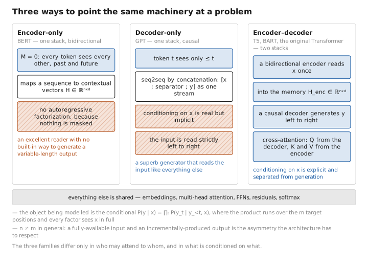
Figure 1. Three ways to point the same machinery at a problem.

3. Why two stacks, precisely

Why not just use the decoder-only concatenation trick, which clearly works (and is what most chat LLMs do)? The encoder–decoder split buys three concrete things, each a direct consequence of treating input and output differently.

(a) Bidirectional encoding of the input. When the entire input is available before generation begins — which is exactly the seq2seq setting — there is no reason to read it left-to-right. A token in the source sentence can be disambiguated by words that come after it. The encoder’s unmasked self-attention lets every input token attend to every other, producing a representation that a causal stream simply cannot match for the input portion. The decoder-only model pays for its uniformity by reading the input causally too.

(b) A reusable, compute-once memory. The encoder runs once per input and produces $H_{\text{enc}}$, which is then frozen for the entire generation. Every one of the $m$ decoding steps attends against the same $H_{\text{enc}}$. We will see in Lesson 9 that this makes the encoder’s keys and values a one-time cost, separate from the per-step decoder cache — a clean computational separation the concatenation approach blurs.

(c) Decoupled lengths and roles. The encoder’s depth, width, and even vocabulary can differ from the decoder’s; the two stacks specialize, one as a reader and one as a writer. The cost is the extra cross-attention sublayer and a more complex architecture — which is the entire subject of Lessons 4–5.

Invariant (the whole course in one line). The encoder compresses context into $H_{\text{enc}}$; the decoder generates $y$ conditioned on it; cross-attention is the only mechanism that did not already exist in a decoder-only model. If you internalize one sentence, make it this one.

---

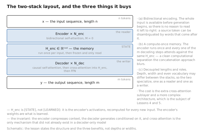
Figure 2. The two-stack layout, and the three things it buys.

4. The function signature and the three number-categories

Formally, an encoder–decoder model is a pair of maps sharing the parameter vector $\theta\in\mathbb R^P$:

$$ \underbrace{\mathrm{Enc}:\ \mathcal V_x^{\le n}\times\Theta \to \mathbb R^{n\times d}}_{x\,\mapsto\,H_{\text{enc}}}, \qquad \underbrace{\mathrm{Dec}:\ \mathcal V_y^{\lt t}\times \mathbb R^{n\times d}\times\Theta \to \Delta^{V_y-1}}_{(y_{\lt t},\,H_{\text{enc}})\,\mapsto\,\hat{\mathbf p}_t}, $$

where the decoder emits a categorical distribution $\hat{\mathbf p}_t$ over the output vocabulary on the probability simplex $\Delta^{V_y-1}$. The encoder is evaluated once; the decoder is evaluated $m$ times, each time reading the same $H_{\text{enc}}$ and one more output token. The parameter vector $\theta$ now contains three groups instead of the decoder-only model’s one: encoder parameters, decoder parameters (which include the extra cross-attention projections), and the shared/​tied embeddings.

As in the decoder-only course, every number in this course belongs to exactly one category:

• [LEARNED] — $\theta$: encoder and decoder weight matrices, the cross-attention projections $W_Q^{\text{cross}},W_K^{\text{cross}},W_V^{\text{cross}}$, embeddings, the output head.
• [CONFIG] — architecture and process: encoder/decoder depths $N_{\text{enc}},N_{\text{dec}}$, width $d$, head count $h$, the masking patterns, the pretraining objective’s corruption rate, beam width.
• [STATE] — transient: $H_{\text{enc}}$ itself (a function of the current input!), the decoder self-attention KV cache, the cross-attention KV cache, logits, attention matrices.

Note one subtlety that recurs throughout: $H_{\text{enc}}$ is [STATE], not [LEARNED]. It looks like a fixed thing during generation, but it is recomputed for every new input — it is the encoder’s activations, not its weights. The encoder’s weights are [LEARNED]; the memory it produces is [STATE].

---

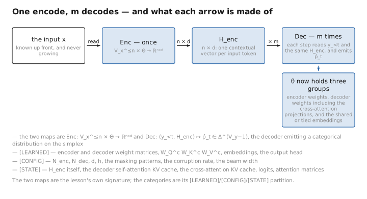
Figure 3. One encode, m decodes — and what each arrow is made of.

5. What is genuinely new — and what is not

It is worth drawing the line now, because the rest of the course lives on it. From the decoder-only model you already have, an encoder–decoder transformer reuses unchanged: token embeddings, positional information, scaled dot-product self-attention, multi-head structure, the FFN/MLP sublayer, residual connections and normalization, the softmax output head, and cross-entropy training with teacher forcing. It adds exactly one new operation — cross-attention (Lesson 4) — and rearranges masking (the encoder drops the causal mask; the decoder keeps it) and the training objective (denoising pretraining instead of plain next-token prediction; Lesson 7). That is the entire delta. The lessons ahead are mostly about getting those three changes exactly right.

---

Conclusion

A sequence-to-sequence task asks for a conditional distribution $P_\theta(y\mid x)=\prod_t P_\theta(y_t\mid y_{\lt t},x)$ in which the input $x$ is fully available and the output $y$ is generated left to right. That asymmetry motivates two stacks: a bidirectional encoder that reads $x$ once into a memory $H_{\text{enc}}\in\mathbb R^{n\times d}$, and a causal decoder that generates $y$ while attending to that memory through cross-attention. Encoder-only models read but do not generate; decoder-only models generate but read causally and implicitly; the encoder–decoder keeps the two roles separate. Everything in the architecture is inherited from the decoder-only transformer except one new mechanism (cross-attention), one rearrangement of masks, and one change of objective. And $H_{\text{enc}}$, the heart of the conditioning, is [STATE] — recomputed per input, never a parameter.

We open the box bottom-up, starting with the reader. Lesson 2 builds the encoder stack and shows what dropping the causal mask actually buys.

---

← Previous: (none — this is the first lesson) · Course index · Next: Lesson 2 — The Encoder Stack →

Appendices: A — Formulas · B — Architecture Comparison · C — Acronyms

---

The figures in this lesson follow the shared figure key , which explains what every shape, line style and colour means.