Lesson 2 — The Encoder Stack: Bidirectional Context
Technical course on encoder–decoder transformers — Lesson 2 of 10.
Recap of Lesson 1
A seq2seq model is the conditional map $P_\theta(y\mid x)=\prod_t P_\theta(y_t\mid y_{\lt t},x)$: the input $x$ is fully available, the output $y$ is generated left to right. That asymmetry motivates two stacks — a bidirectional encoder that reads $x$ once into a memory $H_{\text{enc}}\in\mathbb R^{n\times d}$ (which is [STATE], recomputed per input), and a causal decoder that generates conditioned on it via cross-attention, the one genuinely new mechanism. We now build the first stack and make precise what dropping the causal mask buys.
1. The encoder’s one job: compress $x$ into a memory
The encoder is a reader. It takes the input token sequence $x=(x_1,\dots,x_n)$, embeds it into $H^{(0)}\in\mathbb R^{n\times d}$ exactly as a decoder-only model would (token embedding $E_x\in\mathbb R^{V_x\times d}$ plus positional information), and runs it through $N_{\text{enc}}$ transformer blocks to produce
$$ H_{\text{enc}}:=H^{(N_{\text{enc}})}\in\mathbb R^{n\times d}. $$That is the entire output of the encoder — one contextual vector per input token, not a single pooled vector. This matters: the decoder will attend over all $n$ of these rows individually (Lesson 4), so the “compression” is not into a fixed-size bottleneck but into a length-$n$ set of context-rich vectors. (The single-vector bottleneck was exactly the limitation of pre-attention RNN seq2seq models that attention was invented to remove.) Once produced, $H_{\text{enc}}$ is frozen for the whole of generation — it is computed in a single forward pass and then only read.
2. Bidirectional self-attention: the missing mask
Here is the one structural difference between an encoder block and the decoder-only block you know. Recall scaled dot-product attention:
$$ \mathrm{Attn}(Q,K,V)=\mathrm{softmax}\!\Big(\tfrac{QK^\top}{\sqrt{d_k}}+M\Big)V, \qquad Q=HW_Q,\ K=HW_K,\ V=HW_V . $$In a decoder-only model the mask $M$ is the $-\infty$ upper-triangular causal mask: position $i$ may not attend to $j\gt i$. The encoder simply sets $M=0$ (apart from padding, §4). Every input token attends to every other — past and future:
$$ M^{\text{enc}}_{ij}=0\ \ \forall i,j \quad\Longrightarrow\quad A_{ij}\gt 0\ \text{for all } i,j,\qquad A\mathbf 1=\mathbf 1. $$The attention matrix $A\in\mathbb R^{n\times n}$ is now full (dense, row-stochastic) rather than lower-triangular. Mechanically the change is trivial — delete the mask. Conceptually it is the reason the encoder exists. Because the input is known in full before any output token is produced, there is no notion of “future leakage” to prevent: letting token $i$ see token $j\gt i$ does not cheat any prediction, because the encoder predicts nothing. It only represents.
Why this helps is concrete. Consider encoding the English source “the bank of the river” for translation. The correct sense of “bank” is fixed by “river,” which appears after it. A causal reader processing “the bank” has not yet seen “river” and must commit to a representation prematurely; the bidirectional encoder lets “bank” attend forward to “river” and resolve the ambiguity in the same layer. Every downstream cross-attention then reads a “bank” vector that already knows it is a riverbank.
Everything else inside the block — the $\sqrt{d_k}$ scaling (the same variance argument: raw logits have standard deviation $\sqrt{d_k}$, so we rescale to keep softmax out of its zero-gradient saturation regime), the softmax Jacobian $\mathrm{diag}(\mathbf a)-\mathbf a\mathbf a^\top$, multi-head structure with $d_k=d/h$ — is identical to what you already know. Only $M$ changed.
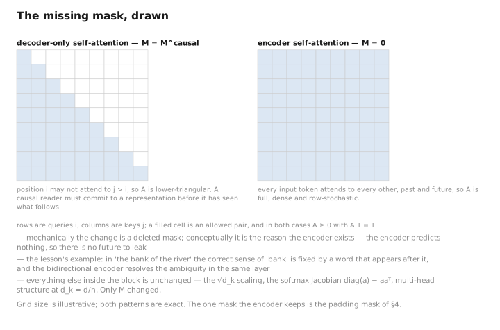
Figure 1. The missing mask, drawn.
3. The encoder block
One encoder block is two pre-norm residual sublayers — multi-head bidirectional self-attention and a position-wise FFN — exactly the standard transformer block minus the causal mask:
$$ \begin{aligned} H' &= H + \mathrm{MHA}_{\text{bidir}}\big(\mathrm{Norm}(H)\big),\\ H^{\text{out}} &= H' + \mathrm{FFN}\big(\mathrm{Norm}(H')\big), \end{aligned} \qquad \mathrm{FFN}(\mathbf x)=W_2\,\phi(W_1\mathbf x+\mathbf b_1)+\mathbf b_2,\ \ d_{ff}\approx 4d . $$The residual gives the by-now-familiar layer Jacobian $I+\partial\mathcal F$ — an identity gradient path that makes deep stacks trainable. Stacking $N_{\text{enc}}$ such blocks yields $H_{\text{enc}}$. The parameter budget per encoder block is the usual $\approx 4d^2$ (attention: $W_Q,W_K,W_V,W_O$) $+\ \approx 8d^2$ (FFN) $=12d^2$; there is no cross-attention here — cross-attention lives only in the decoder.
Note (what an encoder block is not). It is not a “smaller decoder.” It has two sublayers, not three; it never sees the output sequence; and it produces representations, not a probability distribution. There is no output head on the encoder of a standard T5/BART model.
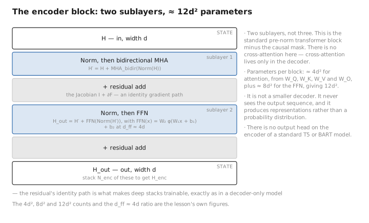
Figure 2. The encoder block: two sublayers, ≈ 12d² parameters.
4. Padding masks: the mask that does survive
We said the encoder drops the causal mask. It keeps a different one. Real batches contain sequences of different lengths $n$, padded to a common length with a special <pad> token. Those pad positions carry no information and must not be attended to, or they would leak meaningless vectors into every real token’s representation. So the encoder uses a padding mask: for each query $i$, any key position $j$ that is padding gets $M_{ij}=-\infty$.
This is [CONFIG] in the sense of being a deterministic function of the input lengths, with zero parameters — but unlike the causal mask it depends on the data (which positions are padding), so in practice it travels with the batch as [STATE]. The same encoder padding mask is reused later by the decoder’s cross-attention (Lesson 4), so that generated tokens never attend to padded input positions. Keep it in mind: it is the one mask the encoder carries forward into the rest of the model.
5. Is the encoder just BERT?
Architecturally, an encoder stack with bidirectional self-attention is essentially BERT’s stack — and that is a useful anchor. But two differences matter for our story:
- No MLM head, no
[CLS]objective. BERT is trained with a masked-language-model head and used standalone for classification via a pooled[CLS]vector. The T5/BART encoder has no such head; it is trained jointly with the decoder on a seq2seq reconstruction objective (Lesson 7), and its output $H_{\text{enc}}$ exists only to be consumed by cross-attention. The encoder is a component, not a finished model. - It produces all $n$ vectors for attention, not a pooled summary. Sentence-embedding uses of BERT often pool $H$ to one vector; the encoder–decoder keeps all $n$ rows precisely so the decoder can attend to different source positions at different output steps (the alignment behavior of Lesson 9).
So: same self-attention machinery as BERT, different role. The encoder is the half of a seq2seq model that does the “reading,” and it reads bidirectionally because it can.
Learned / config / state
| Quantity | Category |
|---|---|
| Embedding $E_x$; per-block $W_Q,W_K,W_V,W_O,W_1,W_2,\gamma,\beta$ | [LEARNED] |
| Depth $N_{\text{enc}}$, width $d$, heads $h$, $d_{ff}$, bidirectional ($M=0$) policy | [CONFIG] |
| Padding mask pattern (data-dependent) | [CONFIG]/[STATE] |
| Hidden states $H^{(\ell)}$, attention matrices $A$, the memory $H_{\text{enc}}$ | [STATE] |
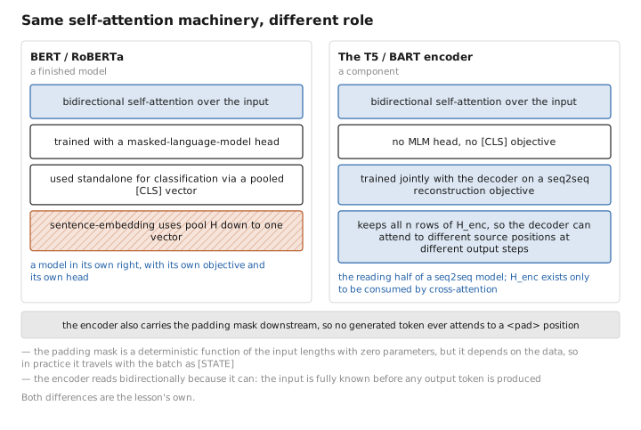
Figure 3. Same self-attention machinery, different role.
Conclusion
The encoder is the reader. It embeds $x$ and runs $N_{\text{enc}}$ standard transformer blocks whose only deviation from the decoder-only block is a deleted causal mask: self-attention is bidirectional ($M=0$), so every input token is contextualized by the whole input, past and future — the right thing to do when the input is fully known. It keeps a padding mask so pad tokens are never attended to, and it passes that mask downstream. Its output is the memory $H_{\text{enc}}\in\mathbb R^{n\times d}$: one contextual vector per input token, computed once and then frozen — and it is [STATE], the encoder’s activations, not its weights. Architecturally it is BERT’s stack, but it carries no output head and exists only to feed cross-attention.
We now have a reader. Next we build the writer — the decoder stack — and see what its causal self-attention shares with a decoder-only model, and what extra sublayer it grows to consume the memory we just built.
← Lesson 1 — Why Two Stacks? · Course index · Next: Lesson 3 — The Decoder Stack →
Appendices: A — Formulas · B — Architecture Comparison · C — Acronyms
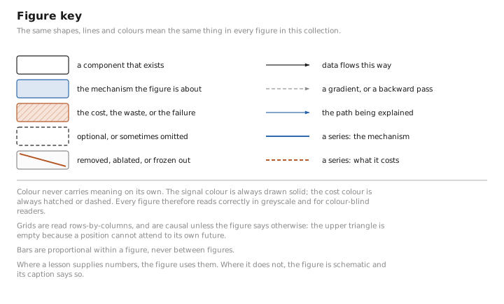
The figures in this lesson follow the shared figure key , which explains what every shape, line style and colour means.