Lesson 3 — The Decoder Stack: Causal Self-Attention Revisited

Technical course on encoder–decoder transformers — Lesson 3 of 10.

---

Recap of Lesson 2

The encoder reads $x$ with bidirectional self-attention ($M=0$) and emits the memory $H_{\text{enc}}\in\mathbb R^{n\times d}$ — one contextual vector per input token, computed once, frozen for generation, and tagged [STATE]. It keeps a padding mask so pad positions are never attended to, and passes that mask downstream. Its only deviation from a decoder-only block was a deleted causal mask. We now build the writer, whose self-attention keeps the causal mask but which grows one extra sublayer to consume the memory.

---

1. The decoder’s job and its two sources of information

The decoder generates the output $y=(y_1,\dots,y_m)$ one token at a time, modeling $P_\theta(y_t\mid y_{\lt t},x)$. To do that it must combine two information streams at every position:

• the output so far $y_{\lt t}$ — what it has already written, read causally;
• the input $x$ — read through the memory $H_{\text{enc}}$, in full.

A decoder-only model has only the first stream (it folds the input into $y_{\lt t}$ by concatenation). The encoder–decoder decoder keeps the first and adds a separate pathway for the second. That separate pathway is cross-attention, and the need for it is precisely why the decoder block has three sublayers where the encoder block had two. This lesson sets up the causal-self-attention sublayer (which you already know) and the slot the cross-attention sublayer occupies; Lesson 4 derives cross-attention itself.

---

2. Causal self-attention, unchanged

The decoder’s first sublayer is ordinary masked multi-head self-attention over the output sequence — bit-for-bit the mechanism from a decoder-only model. Let $H_{\text{dec}}\in\mathbb R^{m\times d}$ be the decoder’s current hidden states (rows = output positions). Then

$$ \mathrm{SelfAttn}(H_{\text{dec}})=\mathrm{softmax}\!\Big(\tfrac{Q_sK_s^\top}{\sqrt{d_k}}+M^{\text{causal}}\Big)V_s, \quad Q_s,K_s,V_s = H_{\text{dec}}W_Q^s,\,H_{\text{dec}}W_K^s,\,H_{\text{dec}}W_V^s, $$

with the same $-\infty$ upper-triangular causal mask as before:

$$ M^{\text{causal}}_{ij}=\begin{cases}0,& j\le i\\ -\infty,& j\gt i\end{cases} $$

This enforces that output position $i$ attends only to $y_{\le i}$, which is exactly what makes the output factorization $\prod_t P_\theta(y_t\mid y_{\lt t},x)$ valid and lets all $m$ output positions be trained in parallel from one forward pass (Lesson 8). Nothing here is new. The superscript $s$ marks these as the self-attention projections, to distinguish them from the cross-attention projections of the next lesson — the decoder owns two complete sets of $W_Q,W_K,W_V$.

---

3. Where cross-attention sits: the three-sublayer block

A decoder block is the standard two-sublayer block with a cross-attention sublayer inserted in the middle:

$$ \begin{aligned} H_1 &= H_{\text{dec}} + \mathrm{SelfAttn}_{\text{causal}}\big(\mathrm{Norm}(H_{\text{dec}})\big), && \text{(1) read the output so far}\\ H_2 &= H_1 + \mathrm{CrossAttn}\big(\mathrm{Norm}(H_1),\,H_{\text{enc}}\big), && \text{(2) read the input memory}\\ H_3 &= H_2 + \mathrm{FFN}\big(\mathrm{Norm}(H_2)\big). && \text{(3) per-position transform} \end{aligned} $$

Each is a pre-norm residual sublayer, so the gradient still flows along an identity path through all three. The ordering is deliberate and standard: the decoder first integrates what it has written (self-attention), then consults the source (cross-attention), then transforms. The cross-attention sublayer is the only one that takes a second argument, $H_{\text{enc}}$ — the same memory for every block and every step.

Compared with a decoder-only block, the decoder block adds exactly sublayer (2) and its parameters $\{W_Q^{c},W_K^{c},W_V^{c},W_O^{c}\}$ and norm. That is the entire architectural cost of conditioning on a separately-encoded input.

---

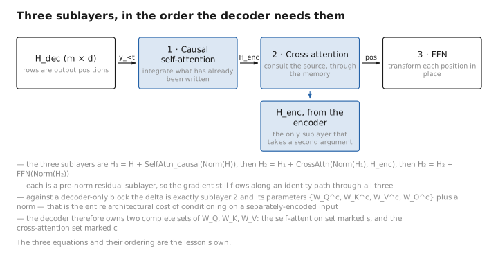
Figure 1. Three sublayers, in the order the decoder needs them.

4. Decoder vs. decoder-only model: the precise delta

It is worth tabulating what actually differs, because the temptation is to imagine the decoder is some exotic object. It is not — it is a decoder-only stack with one sublayer added per block.

Aspect	Decoder-only model	Encoder–decoder decoder
Self-attention	causal	causal (identical)
Conditioning on input	implicit, via concatenated prefix	explicit, via cross-attention to $H_{\text{enc}}$
Sublayers per block	2 (self-attn, FFN)	3 (self-attn, cross-attn, FFN)
Sees the input how	as earlier tokens in the same causal stream	bidirectionally, through the encoder
Output head	over the (single) vocabulary	over the output vocabulary $V_y$

The output head itself is the familiar one: a final norm and an unembedding $W_U\in\mathbb R^{d\times V_y}$ map the top decoder state $\mathbf h_t$ to logits $\mathbf z_t=\mathbf h_t^\top W_U$, then softmax to $\hat{\mathbf p}_t\in\Delta^{V_y-1}$. T5 and BART tie $W_U$ to the (shared) embedding to save $V_y d$ parameters, just as decoder-only models often do. The training loss and the $\partial\mathcal L/\partial\mathbf z=\hat{\mathbf p}-\mathbf y$ gradient identity are unchanged (Lesson 8).

---

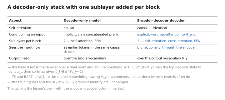
Figure 2. A decoder-only stack with one sublayer added per block.

5. Two embeddings or one?

A small but real design choice: the encoder embeds over $\mathcal V_x$ and the decoder over $\mathcal V_y$. When the task is translation between different languages, these could be separate matrices. In practice T5 and BART use a single shared vocabulary and a single shared embedding matrix across encoder input, decoder input, and output head (so $E_x=E_y=E$, and $W_U=E^\top$). This is [CONFIG]: it cuts parameters and works well when a SentencePiece/BPE vocabulary covers all the languages involved. The original Transformer for WMT En–De likewise shared source/target embeddings. Sharing is the default; separate embeddings are the exception for genuinely disjoint vocabularies.

Learned / config / state

Quantity	Category
Self-attn $\{W_Q^s,W_K^s,W_V^s,W_O^s\}$; cross-attn $\{W_Q^c,W_K^c,W_V^c,W_O^c\}$; FFN; norms; $W_U$	[LEARNED]
$N_{\text{dec}}$, $h$, $d$, $d_{ff}$, causal-mask policy, shared-vs-separate embeddings	[CONFIG]
$H_{\text{dec}}^{(\ell)}$, self-attn and cross-attn matrices, logits $\mathbf z_t$, probabilities $\hat{\mathbf p}_t$	[STATE]

---

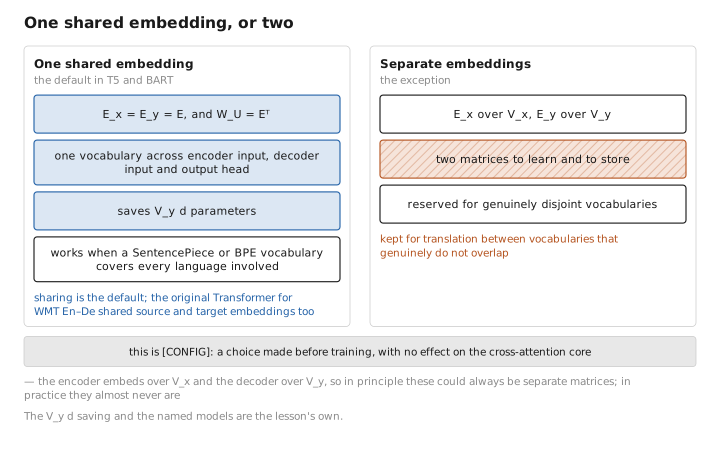
Figure 3. One shared embedding, or two.

Conclusion

The decoder is the writer. Its first sublayer is unchanged causal self-attention over the output so far — the same mechanism, the same $-\infty$ upper-triangular mask, that makes the autoregressive factorization valid. What is new is structural: each decoder block has three sublayers, with a cross-attention sublayer inserted between self-attention and the FFN, and it carries a second full set of attention projections for it. That extra sublayer is the only place the input memory $H_{\text{enc}}$ enters the decoder, and it is the entire architectural cost of explicit conditioning. The output head, weight tying, and loss are inherited intact from the decoder-only model.

We have deferred the one new operation twice now. Lesson 4 derives it from scratch: cross-attention as scaled dot-product attention with its queries and its keys/values drawn from different sequences — and shows why that single change of source is the hinge the whole architecture turns on.

---

← Lesson 2 — The Encoder Stack · Course index · Next: Lesson 4 — Cross-Attention →

Appendices: A — Formulas · B — Architecture Comparison · C — Acronyms

---

The figures in this lesson follow the shared figure key , which explains what every shape, line style and colour means.