Lesson 4 — Cross-Attention: The Only New Mechanism

Technical course on encoder–decoder transformers — Lesson 4 of 10.

---

Recap of Lesson 3

The decoder block has three pre-norm residual sublayers: causal self-attention over the output so far, then cross-attention to the encoder memory, then an FFN. The first and last are inherited unchanged from a decoder-only model; the middle one is the single new operation in the whole architecture, and the decoder carries a second full set of attention projections to run it. We deferred its derivation twice. This lesson pays the debt: cross-attention is scaled dot-product attention with one change — its queries come from the decoder, its keys and values from the encoder.

---

1. The idea: attend to a different sequence

Self-attention computes $Q,K,V$ all from the same input $H$. The entire derivation never required that. Scaled dot-product attention is defined for any three matrices $Q,K,V$ with compatible shapes; the “self” in self-attention is the special case $Q,K,V=HW_Q,HW_K,HW_V$. Cross-attention is the general case: let the queries come from one sequence and the keys/values from another.

In the decoder, the query sequence is the decoder’s own hidden states $H_{\text{dec}}\in\mathbb R^{m\times d}$ (so “what am I, the output token being written, looking for?”), and the key/value sequence is the frozen encoder memory $H_{\text{enc}}\in\mathbb R^{n\times d}$ (so “what does each input token contain, and what information should it contribute?”):

$$ \boxed{\ Q = H_{\text{dec}}\,W_Q^{c}\in\mathbb R^{m\times d_k},\qquad K = H_{\text{enc}}\,W_K^{c}\in\mathbb R^{n\times d_k},\qquad V = H_{\text{enc}}\,W_V^{c}\in\mathbb R^{n\times d_v}.\ } $$

The projections $W_Q^c,W_K^c,W_V^c$ are [LEARNED], distinct from the decoder’s self-attention projections and from the encoder’s. Then the operation is identical in form to everything you know:

$$ \mathrm{CrossAttn}(H_{\text{dec}},H_{\text{enc}})=\mathrm{softmax}\!\Big(\tfrac{QK^\top}{\sqrt{d_k}}+M^{\text{pad}}\Big)V . $$

That is the whole mechanism. The conceptual weight is entirely in where $Q$ and $K,V$ come from — three matrices, two sources.

---

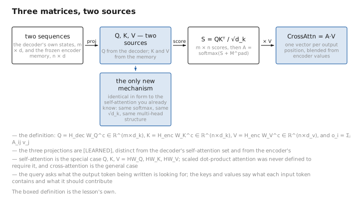
Figure 1. Three matrices, two sources.

2. The shape that gives it away: a non-square attention matrix

In self-attention $Q$ and $K$ have the same number of rows, so the attention matrix is square ($n\times n$ or $m\times m$). In cross-attention the query count $m$ (output length) and the key count $n$ (input length) are different, so the score and attention matrices are rectangular:

$$ S=\frac{QK^\top}{\sqrt{d_k}}\in\mathbb R^{m\times n},\qquad A=\mathrm{softmax}(S+M^{\text{pad}})\in\mathbb R^{m\times n},\qquad \mathrm{CrossAttn}=AV\in\mathbb R^{m\times d_v}. $$

Read the shapes carefully, because they encode the semantics. Row $i$ of $A$ is a distribution over the $n$ input positions — it is “how much output token $i$ attends to each source token.” The softmax is taken over the $n$ key positions (each query row sums to 1: $A\mathbf 1_n=\mathbf 1_m$). The output $AV\in\mathbb R^{m\times d_v}$ has one vector per output position, formed as a convex combination of the input value vectors:

$$ \mathbf o_i=\sum_{j=1}^{n}A_{ij}\,\mathbf v_j,\qquad A_{ij}=\frac{\exp(s_{ij})}{\sum_{k=1}^{n}\exp(s_{ik})},\qquad s_{ij}=\frac{\mathbf q_i^\top\mathbf k_j}{\sqrt{d_k}} . $$

That rectangular $A$ is a soft alignment between output and input — for translation, $A_{ij}$ tends to light up where output word $i$ corresponds to source word $j$ (Lesson 9 makes this concrete). It is the modern, learned, differentiable replacement for the explicit alignment tables of classical statistical machine translation.

---

3. Which masks apply — and which do not

This is the subtlety that trips people up, so state it sharply. Cross-attention uses no causal mask. The decoder may attend to any input position, including ones “after” the current output index — there is no causality between output position $i$ and input position $j$, because they live in different sequences and the entire input is already known. Causality is enforced only in the decoder’s self-attention (Lesson 3); cross-attention is deliberately unmasked in that sense.

What cross-attention does use is the encoder’s padding mask from Lesson 2, applied on the key axis: output tokens must never attend to <pad> positions in the source.

$$ M^{\text{pad}}_{ij}=\begin{cases}0,& x_j\neq\texttt{\textless{}pad\textgreater{}}\\ -\infty,& x_j=\texttt{\textless{}pad\textgreater{}}\end{cases}\quad(\text{same for every output row }i). $$

So the two attention sublayers in a decoder block use different masks: self-attention uses the causal mask (square, lower-triangular), cross-attention uses the source padding mask (rectangular, column-wise). Confusing them is the most common error in implementing a decoder.

---

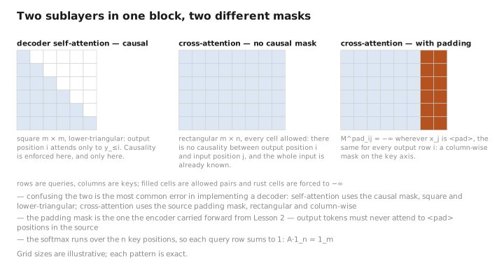
Figure 2. Two sublayers in one block, two different masks.

4. A tiny worked example

Take an output token attending over $n=3$ source tokens, with $d_k=d_v=2$. Suppose the decoder produced query $\mathbf q$ and the encoder memory produced keys/values:

$$ \mathbf q=(1,1),\quad \mathbf k_1=(1,1),\ \mathbf k_2=(1,0),\ \mathbf k_3=(-1,0),\quad \mathbf v_1=(1,0),\ \mathbf v_2=(0,1),\ \mathbf v_3=(1,1). $$

Scores (dot product over $\sqrt{d_k}=\sqrt2\approx1.414$):

$$ s_1=\tfrac{2}{1.414}=1.414,\quad s_2=\tfrac{1}{1.414}=0.707,\quad s_3=\tfrac{-1}{1.414}=-0.707 . $$

Softmax of $(1.414,\,0.707,\,-0.707)$: exponentiate to $(4.11,\,2.03,\,0.49)$, sum $=6.63$, giving the alignment weights

$$ A=(0.620,\ 0.306,\ 0.074),\qquad \textstyle\sum_j A_j=1 . $$

The output token aligns most strongly to source token 1, partly to token 2, and almost ignores token 3 (whose key points away from the query). Output = weighted blend of the input value vectors:

$$ \mathbf o = 0.620\,(1,0)+0.306\,(0,1)+0.074\,(1,1)=(0.694,\ 0.380). $$

Two things to notice. The result is built entirely from encoder values $\mathbf v_j$ — information flows from the input into the output position. And the weights came from comparing a decoder query against encoder keys — the match between what the output is looking for and what each input token offers. That is conditioning on $x$, made differentiable.

---

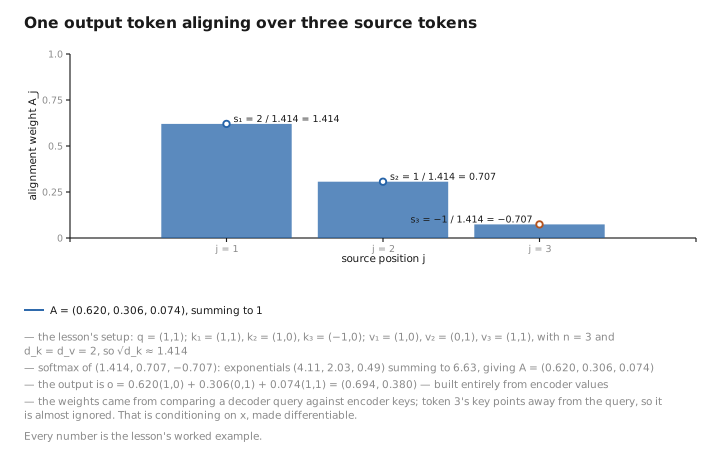
Figure 3. One output token aligning over three source tokens.

5. Gradient flow: cross-attention is the bridge for learning, too

Cross-attention is not only the forward-pass bridge; it is the only path by which a training gradient reaches the encoder. During the backward pass (Lesson 8), the loss is computed at the decoder’s output head. Gradients flow back through the decoder, and at each cross-attention sublayer they split: part updates the decoder’s $W_Q^c$ (through $Q=H_{\text{dec}}W_Q^c$), and part flows through $K=H_{\text{enc}}W_K^c$ and $V=H_{\text{enc}}W_V^c$ into $H_{\text{enc}}$, and from there backward through the entire encoder stack.

$$ \frac{\partial\mathcal L}{\partial H_{\text{enc}}} =\underbrace{\frac{\partial\mathcal L}{\partial K}\frac{\partial K}{\partial H_{\text{enc}}}}_{\text{via }W_K^c} +\underbrace{\frac{\partial\mathcal L}{\partial V}\frac{\partial V}{\partial H_{\text{enc}}}}_{\text{via }W_V^c} \quad\Longrightarrow\quad \text{encoder weights get updated.} $$

This is why the two stacks are trained jointly, end to end, even though only the decoder has a loss head: cut the cross-attention connection and the encoder would receive no learning signal at all. The encoder learns to produce representations useful to the decoder’s queries precisely because the gradient travels this bridge.

Learned / config / state

Quantity	Category
Cross-attn projections $W_Q^c,W_K^c,W_V^c,W_O^c$	[LEARNED]
$\sqrt{d_k}$ scaling, “no causal mask” policy, head count	[CONFIG]
Source padding mask $M^{\text{pad}}$ (data-dependent)	[CONFIG]/[STATE]
Scores $S$, alignment $A\in\mathbb R^{m\times n}$, output $AV$	[STATE]

---

Conclusion

Cross-attention is scaled dot-product attention with one change of source: queries from the decoder, keys and values from the encoder memory, $Q=H_{\text{dec}}W_Q^c$, $K,V=H_{\text{enc}}W_K^c, H_{\text{enc}}W_V^c$. The resulting attention matrix is rectangular ($m\times n$) — a soft, learned alignment whose row $i$ is a distribution over the $n$ input positions, and whose output blends input value vectors into each output position. It uses no causal mask (the input is fully known) but does apply the source padding mask. And it is the sole pathway by which training gradients reach the encoder, which is why the two stacks are learned jointly. Everything about the operation — the softmax, the $\sqrt{d_k}$, the multi-head structure — is what you already knew; only the two sources are new. This is the mechanism the entire course’s invariant names.

With all three sublayers now derived, Lesson 5 assembles them into the complete encoder–decoder block, counts the parameters, draws the whole architecture, and pins down where T5 and BART differ from the textbook version.

---

← Lesson 3 — The Decoder Stack · Course index · Next: Lesson 5 — The Encoder–Decoder Block →

Appendices: A — Formulas · B — Architecture Comparison · C — Acronyms

---

The figures in this lesson follow the shared figure key , which explains what every shape, line style and colour means.