Lesson 5 — The Encoder–Decoder Block & Full Architecture

Technical course on encoder–decoder transformers — Lesson 5 of 10.

---

Recap of Lesson 4

Cross-attention is scaled dot-product attention with queries from the decoder and keys/values from the encoder memory: $Q=H_{\text{dec}}W_Q^c$, $K,V=H_{\text{enc}}W_K^c,H_{\text{enc}}W_V^c$, giving a rectangular alignment $A\in\mathbb R^{m\times n}$ and output $AV\in\mathbb R^{m\times d_v}$. It uses the source padding mask but no causal mask, and it is the sole bridge for the training gradient into the encoder. With all three decoder sublayers derived, we now assemble the full model, count its parameters, and locate where T5 and BART deviate from the textbook Transformer.

---

1. The two block types, side by side

The architecture is built from two block types repeated $N_{\text{enc}}$ and $N_{\text{dec}}$ times. Writing $\mathrm{Norm}$ for the (pre-)normalization:

$$ \textbf{Encoder block:}\quad \begin{aligned} H' &= H + \mathrm{SelfAttn}_{\text{bidir}}(\mathrm{Norm}(H))\\ H^{\text{out}} &= H' + \mathrm{FFN}(\mathrm{Norm}(H')) \end{aligned} $$$$ \textbf{Decoder block:}\quad \begin{aligned} H_1 &= H + \mathrm{SelfAttn}_{\text{causal}}(\mathrm{Norm}(H))\\ H_2 &= H_1 + \mathrm{CrossAttn}(\mathrm{Norm}(H_1),\,H_{\text{enc}})\\ H_3 &= H_2 + \mathrm{FFN}(\mathrm{Norm}(H_2)) \end{aligned} $$

The encoder block has two sublayers; the decoder block has three. Every decoder block consumes the same $H_{\text{enc}}$ — the encoder is run once, and its output is broadcast to all $N_{\text{dec}}$ cross-attention sublayers. This is the structural picture of the course invariant: one compression ($H_{\text{enc}}$), many conditioned generations.

---

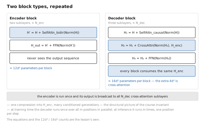
Figure 1. Two block types, repeated.

2. The full forward map

End to end, an encoder–decoder transformer computes:

$$ x \xrightarrow{E_x(+\text{pos})} H^{(0)}_{\text{enc}} \xrightarrow{N_{\text{enc}}\text{ enc blocks}} H_{\text{enc}} $$$$ y_{\lt t} \xrightarrow{E_y(+\text{pos})} H^{(0)}_{\text{dec}} \xrightarrow[\text{each block also reads }H_{\text{enc}}]{N_{\text{dec}}\text{ dec blocks}} H_{\text{dec}} \xrightarrow{W_U} \mathbf z_t \xrightarrow{\mathrm{softmax}} \hat{\mathbf p}_t . $$

The encoder subgraph runs to completion first; then the decoder subgraph runs, every block dipping into $H_{\text{enc}}$. At training time the decoder runs once over all $m$ positions in parallel (Lesson 8); at inference it runs $m$ times, one position per step (Lesson 9).

---

3. Parameter budget

Count parameters per block (ignoring biases and norm gains, which are $O(d)$). Width $d$, FFN width $d_{ff}=4d$.

• Attention sublayer: $W_Q,W_K,W_V,W_O$, each $\approx d\times d$ → $4d^2$.
• FFN sublayer: $W_1\in\mathbb R^{d\times 4d}$, $W_2\in\mathbb R^{4d\times d}$ → $8d^2$.

So an encoder block (1 attention + 1 FFN) is $\approx 12d^2$, and a decoder block (2 attention + 1 FFN) is $\approx 16d^2$ — the extra $4d^2$ is the cross-attention sublayer. The whole model, plus embedding/unembedding:

$$ P \approx \underbrace{12\,N_{\text{enc}}\,d^2}_{\text{encoder}} \;+\; \underbrace{16\,N_{\text{dec}}\,d^2}_{\text{decoder}} \;+\; \underbrace{V d}_{\text{(tied) embedding}} . $$

A useful sanity check against a decoder-only model of the same $d$ and total depth: an encoder–decoder spends $16d^2$ per decoder layer versus $12d^2$ per decoder-only layer, the difference being cross-attention. With the common symmetric choice $N_{\text{enc}}=N_{\text{dec}}=L$, the two stacks together cost $28Ld^2$ — roughly $2.3\times$ a decoder-only model of depth $L$, which is why encoder–decoder models are typically described by their total layer count (e.g. T5-base is “12 + 12”).

---

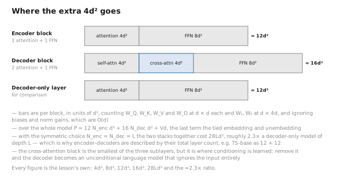
Figure 2. Where the extra 4d² goes.

4. T5 vs. BART: two real instantiations

The textbook is the original 2017 Transformer (Vaswani et al.). T5 and BART are the two encoder–decoder models you will actually meet, and they differ from the textbook — and each other — in instructive, mostly [CONFIG], ways.

BART (Lewis et al., 2019) is deliberately close to the original Transformer: learned absolute positional embeddings, GELU activations, post-style layer norm, and a standard encoder–decoder shape (e.g. BART-large is 12 encoder + 12 decoder layers, $d=1024$). Its novelty is not the architecture but the pretraining objective (Lesson 7). Think of BART as “the original Transformer, pretrained as a denoising autoencoder.”

T5 (Raffel et al., 2019) keeps the same skeleton but makes several specific changes:

• Relative position bias instead of absolute positions. T5 adds a learned scalar bias $b_{i-j}$ (bucketed by relative distance, shared across layers within a stack) directly to the attention logits, and adds no positional embedding at the input: $s_{ij}=\frac{\mathbf q_i^\top\mathbf k_j}{\sqrt{d_k}}+b_{\text{bucket}(i-j)}$. This extrapolates to longer sequences better than learned absolute positions.
• No $\sqrt{d_k}$ scaling in the dot product (T5 folds scale handling into initialization) — a small but real deviation from the boxed formula of Lesson 4. Most other implementations keep the $\sqrt{d_k}$.
• RMSNorm, pre-norm placement, no biases in its dense layers — choices that improve training stability at scale.
• Everything framed as text-to-text (Lesson 10), which is a usage convention, not an architectural one.

The cross-attention mechanism itself is identical in both — the invariant holds regardless of these dressings. What differs is positional handling, normalization, activation, and objective. A reader who knows the original Transformer can read either by patching in these substitutions.

Aspect	Original Transformer	BART	T5
Positions	sinusoidal absolute	learned absolute	relative bias (in logits)
Activation	ReLU	GELU	ReLU (T5), GeGLU (T5 v1.1)
Norm	post-norm LayerNorm	post-norm LayerNorm	pre-norm RMSNorm
Dot-product scale	$1/\sqrt{d_k}$	$1/\sqrt{d_k}$	none (in init)
Pretraining	(trained on MT directly)	denoising (5 noises)	span corruption

---

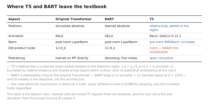
Figure 3. Where T5 and BART leave the textbook.

5. Where the parameters do their work

A closing intuition before training. The encoder’s $12N_{\text{enc}}d^2$ parameters learn to read — to build $H_{\text{enc}}$ rows that expose, to any future query, whatever the decoder might need: word sense, syntactic role, salience for summarization. The decoder’s $16N_{\text{dec}}d^2$ split their labor three ways per block: self-attention parameters track the output written so far, cross-attention parameters learn what to retrieve from the source, and the FFN parameters do the per-position transformation that turns retrieved content into the next-token prediction. The cross-attention block is the smallest of the three ($4d^2$) but it is where conditioning is learned — remove it and the decoder becomes an unconditional language model that ignores the input entirely.

Learned / config / state

Quantity	Category
All block weights (enc + dec), embeddings, $W_U$, T5 relative-position biases	[LEARNED]
$N_{\text{enc}},N_{\text{dec}},d,h,d_{ff}$; position scheme; norm type; activation; scaling policy	[CONFIG]
$H_{\text{enc}}$, $H_{\text{dec}}^{(\ell)}$, all attention matrices, logits	[STATE]

---

Conclusion

The full architecture is two block types repeated: a two-sublayer encoder block ($\approx 12d^2$ params) and a three-sublayer decoder block ($\approx 16d^2$, the extra $4d^2$ being cross-attention), with the encoder run once and its memory $H_{\text{enc}}$ broadcast to every decoder block. Total parameters scale as $12N_{\text{enc}}d^2+16N_{\text{dec}}d^2+Vd$. BART is essentially the original Transformer with a denoising objective; T5 keeps the skeleton but swaps in relative position bias, RMSNorm/pre-norm, and drops the explicit $\sqrt{d_k}$ — all [CONFIG] changes that leave cross-attention, and the course invariant, untouched. The cross-attention sublayer is the architecture’s smallest piece and its conceptual core.

The architecture is now complete. Before training it, Lesson 6 takes a step back to show that this two-stack object is one point on a spectrum: collapse the seam between encoder and decoder with a single clever mask — the prefix-LM — and you recover a one-stack model that behaves almost identically, which is exactly why decoder-only models can do seq2seq at all.

---

← Lesson 4 — Cross-Attention · Course index · Next: Lesson 6 — Prefix-LM →

Appendices: A — Formulas · B — Architecture Comparison · C — Acronyms

---

The figures in this lesson follow the shared figure key , which explains what every shape, line style and colour means.