Lesson 6 — Prefix-LM: Encoder–Decoder as a Special Case
Technical course on encoder–decoder transformers — Lesson 6 of 10.
Recap of Lesson 5
The full model is a stack of two-sublayer encoder blocks and three-sublayer decoder blocks; the encoder runs once into $H_{\text{enc}}$, broadcast to every decoder block’s cross-attention. Parameters scale as $12N_{\text{enc}}d^2+16N_{\text{dec}}d^2+Vd$. T5 and BART differ from the textbook only in [CONFIG] dressings (positions, norm, activation, objective), never in the cross-attention core. We now zoom out: the two-stack design is one point on a spectrum, and a single mask connects it to the decoder-only model.
1. The question: do we need two stacks?
Lesson 1 argued why two stacks help — bidirectional encoding and a compute-once memory. But decoder-only models clearly can do translation and summarization by concatenation. So the honest question is: is the encoder–decoder a fundamentally different object, or a special arrangement of the same one? The answer is the latter, and the bridge is a masking trick called the prefix language model (prefix-LM). Understanding it dissolves the apparent gulf between the two families and explains why the field could later drop encoder–decoders for most tasks without losing capability.
2. The unifying view: it’s all about the mask
Recall that the only thing distinguishing encoder self-attention from decoder self-attention was the mask $M$: $M=0$ (bidirectional) for the encoder, $M=M^{\text{causal}}$ (lower-triangular) for the decoder. Now put input and output into one sequence $[\,x\,;\,y\,]$ of length $n+m$ and run a single stack over it, but with a block-structured mask that gives the input part bidirectional attention and the output part causal attention:
$$ M^{\text{prefix}}_{ij}= \begin{cases} 0, & j\le n \quad\text{(any token may attend to the whole input prefix)}\\[2pt] 0, & n\lt j\le i \quad\text{(output token attends to earlier output)}\\[2pt] -\infty, & j\gt i \text{ and } j\gt n \quad\text{(no peeking at future output)} \end{cases} $$In words: the first $n$ positions (the prefix $x$) are mutually fully visible — like an encoder; positions $n+1\dots n+m$ (the continuation $y$) see the entire prefix and all earlier output but not future output — like a decoder. This is the prefix-LM mask, and it gives a single-stack model the two behaviors the two-stack model split apart.
A model trained this way conditions its generation of $y$ on a bidirectionally-encoded $x$ — the key advantage of the encoder — without a separate stack and without cross-attention. The input is encoded by the same self-attention that generates, just under a more permissive mask for the prefix region.
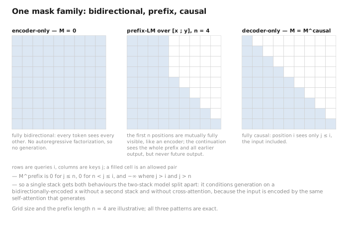
Figure 1. One mask family: bidirectional, prefix, causal.
3. How prefix-LM relates to the two-stack model
The two designs compute closely related functions, and it is worth being precise about what is shared and what differs.
What is shared. Both give $x$ bidirectional context and generate $y$ causally conditioned on all of $x$. Both factorize $P_\theta(y\mid x)=\prod_t P_\theta(y_t\mid y_{\lt t},x)$.
What differs.
- Parameters. The two-stack model has separate weights for reading and writing, plus dedicated cross-attention projections. The prefix-LM reuses one set of weights for both roles and conditions through ordinary self-attention — no $W^c_{Q,K,V}$ at all. Conditioning is “free” in parameter terms but shares capacity between reading and writing.
- Compute reuse. The two-stack encoder produces $H_{\text{enc}}$ once; in a prefix-LM the prefix’s keys/values are likewise computed once and cached, so per-step decoding cost is similar. But the prefix-LM recomputes nothing extra — there is no second stack to run.
- Depth of conditioning. In the two-stack model, conditioning is injected at every decoder layer via cross-attention; in the prefix-LM it is mediated by the shared representation. Empirically the two-stack design tends to be a bit stronger on hard seq2seq tasks (translation, summarization), which is part of why T5 chose it; prefix-LM is competitive and simpler.
So the encoder–decoder is the prefix-LM with the prefix and continuation given their own parameter sets and bonded by cross-attention. Conversely, a prefix-LM is an encoder–decoder with the seam removed and weights tied. They are two points on one design axis.
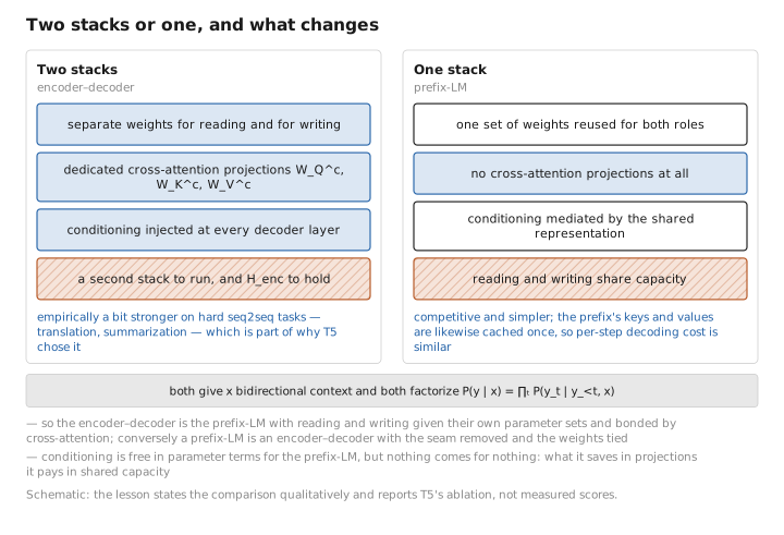
Figure 2. Two stacks or one, and what changes.
4. The full spectrum: one mask family, three architectures
Step back one more notch and the entire landscape of Lesson 1 collapses into a single statement: the three transformer families differ only in their attention mask (and whether $K,V$ come from a second sequence). Everything else is shared.
| Architecture | Mask over the relevant region | Conditioning | Canonical models |
|---|---|---|---|
| Encoder-only | fully bidirectional ($M=0$) | none (it only reads) | BERT, RoBERTa |
| Encoder–decoder | bidirectional enc + causal dec + cross-attn | explicit, per decoder layer | T5, BART, original Transformer |
| Prefix-LM | bidirectional prefix + causal suffix (one stack) | implicit, shared weights | UniLM, T5’s “prefix-LM” baseline, GLM |
| Decoder-only | fully causal | implicit, via concatenated prefix | GPT, Llama, Mistral |
Read top to bottom, the mask grows steadily more causal and the conditioning steadily more implicit. The encoder-only model is “all bidirectional, no generation”; the decoder-only is “all causal, generation by continuation”; the encoder–decoder and prefix-LM sit in between, mixing the two regimes — the former by separating the regimes into two stacks, the latter by splitting one sequence with a block mask.
This is the deep reason a modern decoder-only LLM can translate and summarize despite having no encoder: the causal mask plus a well-chosen prompt approximates the prefix-LM’s behavior, and the prefix-LM approximates the encoder–decoder’s. What the decoder-only gives up — bidirectional input encoding and a clean compute-once memory — turned out to matter less than the simplicity and scaling convenience of a single uniform stack, which is why the field largely consolidated on decoder-only for general-purpose LLMs while keeping encoder–decoders where their inductive bias pays off (Lesson 10).
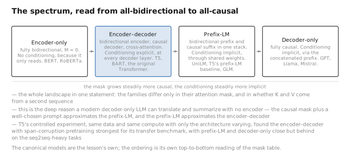
Figure 3. The spectrum, read from all-bidirectional to all-causal.
5. T5’s experiment, briefly
The T5 paper ran exactly this comparison as a controlled experiment — same data, same compute, varying only the architecture/mask — and found the encoder–decoder with span-corruption pretraining the strongest configuration for its transfer-learning benchmark, with the prefix-LM and decoder-only variants close but behind on the seq2seq-heavy tasks. That result is the empirical anchor under this whole lesson: the spectrum is real, the points are genuinely interchangeable in principle, and the two-stack design earns its extra cross-attention parameters on tasks where reading the input well is decisive.
Learned / config / state
| Quantity | Category |
|---|---|
| Shared stack weights (prefix-LM) or separate enc/dec weights (two-stack) | [LEARNED] |
| Choice of mask family (bidirectional / prefix / causal); one-stack vs. two-stack | [CONFIG] |
| The block-structured mask $M^{\text{prefix}}$ (data/length dependent) | [CONFIG]/[STATE] |
| Hidden states, attention matrices | [STATE] |
Conclusion
The encoder–decoder is not a different species — it is one point on a masking spectrum. Put $[\,x\,;\,y\,]$ in a single stack under a prefix-LM mask (bidirectional over the prefix $x$, causal over the continuation $y$) and you condition generation on a bidirectionally-encoded input without a second stack or cross-attention. The encoder–decoder is the prefix-LM with reading and writing given separate parameters and bonded by cross-attention; the decoder-only is the same idea with a fully causal mask and implicit, prompt-based conditioning. All three families — and encoder-only at the far end — differ only in their attention mask and where $K,V$ come from. T5’s own ablation found the two-stack design strongest for seq2seq transfer, which is the empirical reason the architecture earns its keep.
That closes the architectural arc. The remaining lessons are about use: how this object is trained (Lessons 7–8) and how it generates (Lesson 9). We begin with the objective that made T5 and BART work — denoising pretraining — which is where their stories most sharply diverge from both encoder-only MLM and decoder-only next-token prediction.
← Lesson 5 — The Encoder–Decoder Block · Course index · Next: Lesson 7 — Pretraining Objectives →
Appendices: A — Formulas · B — Architecture Comparison · C — Acronyms
The figures in this lesson follow the shared figure key , which explains what every shape, line style and colour means.