Lesson 7 — Pretraining Objectives: Span Corruption vs. Denoising

Technical course on encoder–decoder transformers — Lesson 7 of 10.

---

Recap of Lesson 6

The encoder–decoder is one point on a masking spectrum: a prefix-LM folds the two stacks into one with a block mask (bidirectional prefix, causal suffix), the decoder-only sits at the fully-causal end, and encoder-only at the fully-bidirectional end. All differ only in mask and in whether $K,V$ come from a second sequence. T5’s ablation found the two-stack design strongest for seq2seq transfer. We now enter the training phase and ask: on what objective is a fresh encoder–decoder pretrained? The answer — denoising — is where T5 and BART diverge most from both MLM and next-token prediction.

---

1. The problem: how do you self-supervise two stacks?

A decoder-only model has an obvious free objective: next-token prediction, where the label at position $t$ is simply $x_{t+1}$. An encoder-only model (BERT) has masked-language-modeling: corrupt 15% of tokens, predict them in place. But an encoder–decoder needs an objective that exercises both the bidirectional reader and the autoregressive writer at once, with no human labels — because the whole point of pretraining is to use raw text at $10^{12}$ scale. The unifying idea both T5 and BART adopt is denoising: corrupt the input text in some way, feed the corrupted version to the encoder, and train the decoder to reconstruct the missing/original content autoregressively. The corruption is what creates a (input, output) pair from a single unlabeled document.

The denoising recipe. Encoder reads a corrupted document $\tilde x$; decoder generates the clean (or missing) content $y$. The loss is ordinary cross-entropy on the decoder’s targets — the architecture and loss are unchanged from Lesson 5; only the way we construct $(\tilde x, y)$ from raw text is new.

This single recipe, instantiated two different ways, is T5 and BART.

---

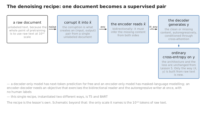
Figure 1. The denoising recipe: one document becomes a supervised pair.

2. T5: span corruption with sentinel tokens

T5’s instantiation is span corruption. Take a document, randomly select spans of tokens totaling a fraction (T5 uses ~15%) of the text, with an average span length of ~3 tokens. Replace each contiguous span with a single unique sentinel token <X>, <Y>, <Z>, … The encoder sees the document with spans collapsed to sentinels; the decoder is trained to emit, for each sentinel, the sentinel followed by the tokens it stood for, ending with a final sentinel.

Concretely, for the original “Thank you for inviting me to your party last week”:

$$ \begin{aligned} \textbf{Encoder input } \tilde x:\quad & \text{Thank you } \texttt{\textless{}X\textgreater{}} \text{ me to your party } \texttt{\textless{}Y\textgreater{}} \text{ week}\\ \textbf{Decoder target } y:\quad & \texttt{\textless{}X\textgreater{}} \text{ for inviting } \texttt{\textless{}Y\textgreater{}} \text{ last } \texttt{\textless{}Z\textgreater{}} \end{aligned} $$

(Here the span “for inviting” became <X> and “last” became <Y>; <Z> marks the end.) Two design payoffs make this clever:

• The target is short. The decoder only generates the corrupted tokens plus sentinels, not the whole document — so the sequence the decoder produces is a small fraction of the input length, which makes pretraining cheap relative to reconstructing everything.
• It exercises both stacks correctly. The encoder must build bidirectional representations rich enough to infer the missing spans from both sides (the word after a sentinel matters as much as the word before — exactly the bidirectional advantage of Lesson 2), and the decoder must generate them in order, conditioned via cross-attention.

The sentinels are added to the vocabulary as ordinary [LEARNED] embeddings; the corruption rate (15%) and mean span length (3) are [CONFIG]; which spans get corrupted on a given example is sampled, i.e. [STATE] for that batch.

---

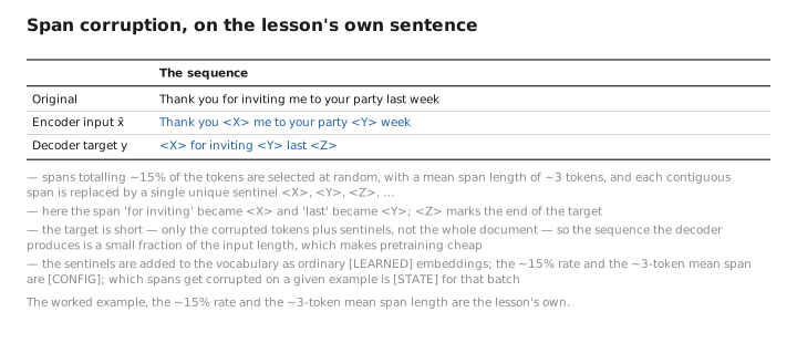
Figure 2. Span corruption, on the lesson’s own sentence.

3. BART: five flavors of noise

BART generalizes denoising into a family of corruptions, and notably allows ones that change the sequence length — which only an encoder–decoder (with its decoupled input/output lengths, Lesson 1) can cleanly handle. BART’s decoder always reconstructs the entire original document, which is more expensive than T5’s span-only target but makes the model a true denoising autoencoder. The five noises:

1. Token masking — replace random tokens with <mask> (BERT-style), but predict the whole document, not just the masked slots.
2. Token deletion — delete random tokens; the model must figure out where something is missing as well as what.
3. Text infilling — replace spans (sampled lengths, including length 0) with a single <mask> each — close to T5’s span idea, and BART found this the most important noise.
4. Sentence permutation — shuffle the order of sentences; the decoder must restore the original order.
5. Document rotation — rotate the document to start at a random token; the model must find the true start.

Infilling and sentence permutation, used together, gave BART its best downstream results. The variety is the point: by forcing the model to undo many kinds of damage, the encoder learns robust representations and the decoder learns fluent generation — which is exactly the pair of skills summarization and translation need.

---

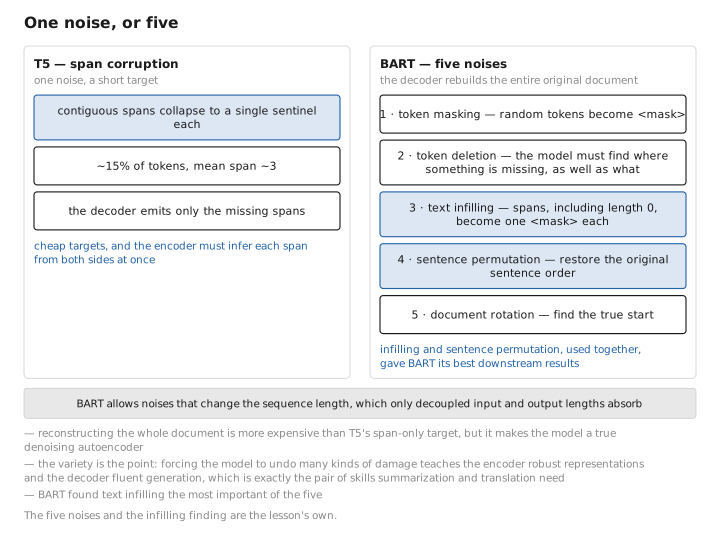
Figure 3. One noise, or five.

4. The loss is the same CE you already know

Whatever the corruption, the training loss is the ordinary teacher-forced cross-entropy over the decoder’s target positions (Lesson 8 details teacher forcing):

$$ \mathcal L(\theta)=-\frac{1}{|y|}\sum_{t=1}^{|y|}\log P_\theta\big(y_t\mid y_{\lt t},\,\tilde x\big) =-\frac{1}{|y|}\sum_{t}\log \hat p_{\,t,\,y_t}, $$

and the logit gradient is the familiar $\partial\mathcal L/\partial\mathbf z_t=\hat{\mathbf p}_t-\mathbf y_t$ (predicted minus one-hot target), which seeds backprop through the decoder, across the cross-attention bridge, and into the encoder (Lesson 4 §5). Nothing about the optimization is special to encoder–decoders; AdamW, warmup-cosine schedules, and gradient clipping carry over unchanged. The objective lives entirely in how $(\tilde x, y)$ is built.

---

5. Contrast with the other two families

It helps to line all three self-supervised objectives up, because they are often conflated.

Family	Objective	What predicts what	Generates?
Encoder-only (BERT)	MLM: mask ~15% in place	bidirectional encoder predicts masked tokens at their positions	no — fills blanks, no autoregression
Decoder-only (GPT)	Next-token CE	causal stack predicts $x_{t+1}$ from $x_{\le t}$	yes, but no separate input encoding
Encoder–decoder (T5/BART)	Denoising / span corruption	encoder reads corrupted $\tilde x$; decoder autoregressively generates clean content	yes, conditioned on bidirectional encoding

The encoder–decoder objective is, in a sense, MLM and next-token prediction fused: like MLM it corrupts and reconstructs and rewards bidirectional reading; like next-token prediction it generates autoregressively. That fusion is only possible because the architecture has both a bidirectional reader and an autoregressive writer joined by cross-attention. The objective and the architecture are made for each other — which is why “span corruption on a decoder-only model” or “next-token prediction on BERT” are not natural things to do, while denoising on an encoder–decoder is.

Learned / config / state

Quantity	Category
Sentinel/<mask> token embeddings, all model weights	[LEARNED]
Corruption type, rate (~15%), mean span length, noise mix	[CONFIG]
Which tokens/spans are corrupted on a given example; the resulting $(\tilde x,y)$	[STATE]
Logits, probabilities, attention matrices	[STATE]

---

Conclusion

Encoder–decoders are pretrained by denoising: corrupt a raw document into $\tilde x$, feed it to the bidirectional encoder, and train the autoregressive decoder to reconstruct the clean or missing content $y$ — turning unlabeled text into supervised pairs with no human annotation. T5 uses span corruption (contiguous spans → single sentinel tokens; the decoder emits only the missing spans, keeping targets short), while BART mixes five noises (masking, deletion, infilling, sentence permutation, document rotation) and reconstructs the whole document. Either way the loss is the ordinary teacher-forced cross-entropy with the familiar $\hat{\mathbf p}-\mathbf y$ logit gradient — the objective’s novelty is purely in how the (corrupted input, clean output) pair is built. The recipe fuses MLM’s bidirectional reconstruction with next-token generation, which is precisely the pair of stacks the architecture provides.

We have the objective. Lesson 8 turns it into a training procedure: teacher forcing, the shifted decoder inputs, training all output positions in parallel, the gradient’s path through cross-attention, and the exposure-bias gap that sets up inference.

---

← Lesson 6 — Prefix-LM · Course index · Next: Lesson 8 — Training: Teacher Forcing →

Appendices: A — Formulas · B — Architecture Comparison · C — Acronyms

---

The figures in this lesson follow the shared figure key , which explains what every shape, line style and colour means.