Lesson 8 — Training: Teacher Forcing & the Loss
Technical course on encoder–decoder transformers — Lesson 8 of 10.
Recap of Lesson 7
Encoder–decoders are pretrained by denoising: corrupt a document into $\tilde x$, encode it bidirectionally, and have the decoder autoregressively reconstruct the clean/missing content $y$. T5 uses span corruption (sentinels, short targets); BART mixes five noises and rebuilds the whole document. Either way the loss is cross-entropy over decoder targets with the gradient $\hat{\mathbf p}-\mathbf y$. We now make the training procedure precise — how the decoder is fed and scored — and draw the sharp line between how the model is trained and how it later generates.
1. The tension: autoregression vs. parallel training
The decoder is autoregressive: $P_\theta(y_t\mid y_{\lt t},x)$ depends on the previous output tokens. At inference those previous tokens are the model’s own (yet-to-be-generated) outputs, so generation is inherently sequential. But at training time we already know the entire correct output $y$ — it is the target. So we can sidestep the sequentiality entirely: feed the decoder the ground-truth previous tokens at every position, rather than its own predictions. This is teacher forcing, and it is what lets us train all $m$ output positions in a single parallel forward pass instead of $m$ sequential ones.
Teacher forcing. During training, the decoder’s input at position $t$ is the true token $y_{t-1}$, not the model’s prediction $\hat y_{t-1}$. The model is always conditioned on a correct prefix, so every position can be computed at once.
2. Shifted inputs and the causal mask, working together
Mechanically, teacher forcing is implemented by feeding the decoder the target sequence shifted right by one, prepended with a start token (<bos> / T5’s <pad>-as-start):
Position $t$ of the decoder receives $y_{t-1}$ as input and is asked to predict $y_t$. The decoder’s causal self-attention mask (Lesson 3) is what makes this safe in parallel: even though the entire shifted target is fed in at once, position $t$ can only attend to inputs $\le t$, so it physically cannot see $y_t$ or later — no label leakage. The combination is the whole trick:
- teacher forcing supplies the correct prefix (so we don’t need to generate), and
- the causal mask prevents any position from peeking at its own answer (so parallel ≠ cheating).
Meanwhile cross-attention attends over the full $H_{\text{enc}}$ with no causal mask — correct, because the input is fully known at every step regardless of the output position.
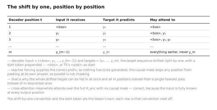
Figure 1. The shift by one, position by position.
3. The loss, summed over positions
With the shifted setup, one forward pass yields $m$ logit vectors $\{\mathbf z_t\}$, hence $m$ predictions, and the loss averages cross-entropy over them:
$$ \mathcal L(\theta)=-\frac{1}{m}\sum_{t=1}^{m}\log P_\theta(y_t\mid y_{\lt t},x) =-\frac{1}{m}\sum_{t=1}^{m}\log\big[\mathrm{softmax}(\mathbf z_t)\big]_{y_t}. $$Just as in the decoder-only case, the per-logit gradient is the clean residual
$$ \frac{\partial\mathcal L}{\partial\mathbf z_t}=\hat{\mathbf p}_t-\mathbf y_t\quad(\text{predicted}-\text{one-hot target}), $$and padding positions in the target (from batching variable-length outputs) are excluded from the average via a target mask — they contribute no loss and no gradient. For fine-tuning on supervised pairs (Lesson 10) the same loss applies with $(x,y)$ the real source/target instead of a corrupted/clean pair; only the data changes.
4. The gradient’s journey: through cross-attention into the encoder
This is the part unique to two-stack training, and Lesson 4 §5 promised the detail. The loss lives only at the decoder’s output head, yet the encoder must learn. Backpropagation routes the signal like this:
$$ \hat{\mathbf p}_t-\mathbf y_t \ \xrightarrow{W_U}\ \frac{\partial\mathcal L}{\partial H_{\text{dec}}} \ \xrightarrow{\text{dec blocks}}\ \frac{\partial\mathcal L}{\partial(\text{cross-attn }K,V)} \ \xrightarrow{W_K^c,\,W_V^c}\ \frac{\partial\mathcal L}{\partial H_{\text{enc}}} \ \xrightarrow{\text{enc blocks}}\ \frac{\partial\mathcal L}{\partial(\text{encoder weights})}. $$Every decoder block contributes a term to $\partial\mathcal L/\partial H_{\text{enc}}$ through its cross-attention $K,V$ projections; these sum, and the total flows backward through the whole encoder. So the two stacks are optimized jointly, end to end in one backward pass — the encoder’s gradient is entirely mediated by cross-attention. This is the precise sense in which “cross-attention is the only new mechanism” governs training as well as the forward pass: it is the sole channel through which the encoder discovers what representations the decoder needs. (Memory cost mirrors this: training caches activations for both stacks, so an encoder–decoder’s activation memory exceeds a decoder-only model’s of comparable decoder size.)
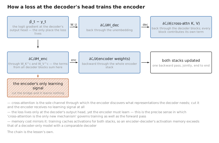
Figure 2. How a loss at the decoder’s head trains the encoder.
5. Training vs. inference: the gap that matters
We can now state the two phases side by side, because their difference drives the next lesson.
| Training (this lesson) | Inference (Lesson 9) | |
|---|---|---|
| Decoder input at $t$ | ground-truth $y_{t-1}$ (teacher forcing) | model’s own previous output $\hat y_{t-1}$ |
| Positions computed | all $m$ at once (parallel) | one at a time (sequential) |
| Encoder runs | once per example | once per example |
| Loss / gradient | yes (writes $\theta$) | none ($\theta$ frozen) |
| Output prefix is | always correct | possibly already wrong |
The last row is the seed of exposure bias: the model is only ever trained on correct prefixes, but at inference it must condition on its own prefixes, which may contain errors it never saw during training. A single early mistake can push the decoder into a region of prefix-space it was never optimized on, and errors compound. Teacher forcing buys parallel, stable training at the cost of this train/test mismatch. Mitigations (scheduled sampling, sequence-level objectives, or just large-scale pretraining making the model robust) exist, but the standard recipe accepts the gap — and inference-time techniques like beam search (Lesson 9) partly compensate by not committing greedily to a single prefix.
Learned / config / state
| Quantity | Category |
|---|---|
| All weights updated by the backward pass | [LEARNED] |
| Teacher-forcing policy, shift-by-one convention, start token, LR schedule, batch size | [CONFIG] |
| Target padding mask (data-dependent) | [CONFIG]/[STATE] |
| Logits $\mathbf z_t$, cached activations (both stacks), gradients, optimizer moments | [STATE] |
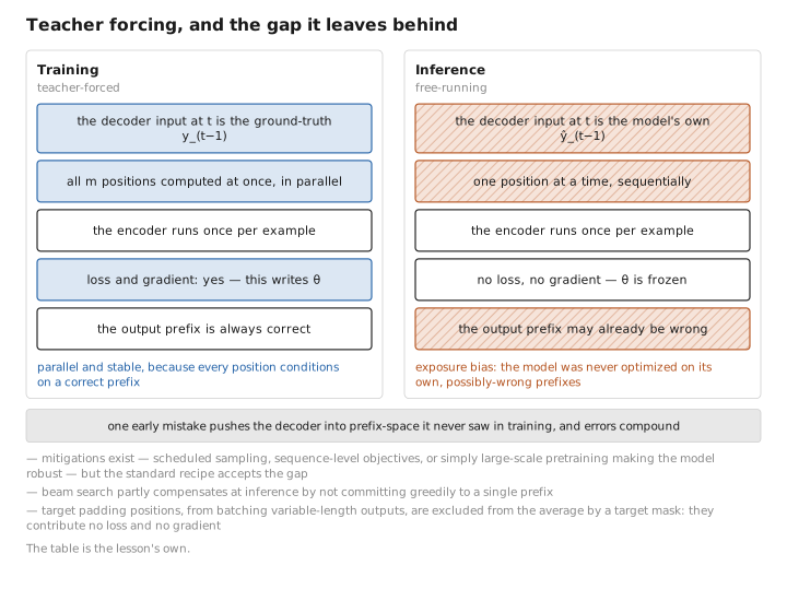
Figure 3. Teacher forcing, and the gap it leaves behind.
Conclusion
Training uses teacher forcing: the decoder is fed the ground-truth output shifted right by one, so every output position conditions on a correct prefix and all $m$ positions can be scored in a single parallel forward pass. The decoder’s causal mask keeps that parallelism honest (no position sees its own target), while cross-attention reads the full encoder memory unmasked. The loss is averaged cross-entropy with the clean $\hat{\mathbf p}_t-\mathbf y_t$ logit gradient, and that gradient flows from the decoder head through cross-attention into the encoder, training both stacks jointly — the encoder’s only learning signal. The price is exposure bias: trained only on correct prefixes, the model must later condition on its own, possibly-wrong outputs.
That mismatch is exactly what the inference phase must manage. Lesson 9 turns the frozen, trained model loose: encode once, decode many, with two distinct KV caches, beam search and length normalization for quality, and coverage and copy mechanisms for the failure modes specific to seq2seq generation.
← Lesson 7 — Pretraining Objectives · Course index · Next: Lesson 9 — Inference →
Appendices: A — Formulas · B — Architecture Comparison · C — Acronyms
The figures in this lesson follow the shared figure key , which explains what every shape, line style and colour means.