Lesson 9 — Inference: Decoding Against a Frozen Memory

Technical course on encoder–decoder transformers — Lesson 9 of 10.

---

Recap of Lesson 8

Training uses teacher forcing: the decoder is fed the ground-truth output shifted right by one, so all $m$ positions are scored in parallel under a causal mask, with cross-attention reading the full encoder memory. The loss is averaged cross-entropy ($\hat{\mathbf p}_t-\mathbf y_t$ gradient), and that gradient is the encoder’s only learning signal, routed through cross-attention. The cost is exposure bias — the model trains on correct prefixes but must later condition on its own. We now run the frozen model: $\theta$ is fixed, no loss, no gradient, only forward passes — and every knob is [CONFIG], every buffer [STATE].

---

1. Encode once, decode many

Inference splits cleanly along the two-stack boundary, and this is where the architecture pays off computationally. The encoder runs exactly once: feed the input $x$, get the memory $H_{\text{enc}}\in\mathbb R^{n\times d}$. Then the decoder runs autoregressively, one token per step, each step attending to $y_{\lt t}$ (self) and to the frozen $H_{\text{enc}}$ (cross):

1. Encode: $H_{\text{enc}}=\mathrm{Enc}(x)$ — once.
2. Start the decoder with $\langle\text{bos}\rangle$.
3. Step $t$: forward the decoder → logits $\mathbf z_t$ → $\hat{\mathbf p}_t=\mathrm{softmax}(\mathbf z_t/T)$ at the last position.
4. Select $y_t$ (strategies below); append it; repeat until <eos> or a length cap.

Unlike training, the decoder cannot be parallelized over output positions — token $t$ genuinely depends on the sampled $y_{t-1}$. But the expensive bidirectional encoding is amortized: it is paid once and reused by all $m$ decoder steps and (for beam search) all beams.

---

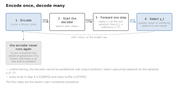
Figure 1. Encode once, decode many.

2. Two KV caches, not one

A decoder-only model caches the keys/values of past tokens to avoid recomputing them each step (the KV cache). An encoder–decoder has two distinct caches, because the decoder runs two kinds of attention:

• Self-attention KV cache — keys/values of the output tokens generated so far. It grows by one each step, exactly like a decoder-only model’s cache. Size $\sim 2\,t\,N_{\text{dec}}\,d$ at step $t$.
• Cross-attention KV cache — keys/values computed from $H_{\text{enc}}$: $K=H_{\text{enc}}W_K^c$, $V=H_{\text{enc}}W_V^c$, per decoder layer. These depend only on the (fixed) input, so they are computed once, right after encoding, and never change during generation. Size $\sim 2\,n\,N_{\text{dec}}\,d$, constant in $t$.

$$ \text{per-step cross-attention cost} = O(n\,d)\ \text{(one query vs. } n\text{ cached encoder keys)}, \quad\text{with }K,V\text{ never recomputed.} $$

This is a concrete efficiency win of the two-stack design: the source representation is encoded once and its cross-attention keys/values are cached once, so each decoding step’s conditioning on the input is cheap and the input is never re-read. The two caches are pure [STATE] — built per request, discarded after.

---

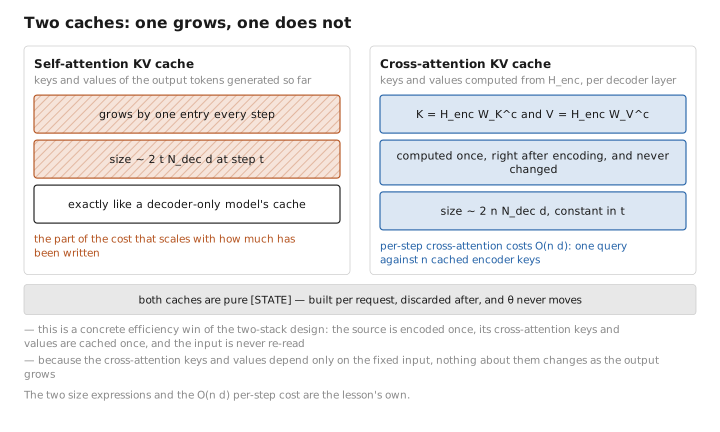
Figure 2. Two caches: one grows, one does not.

3. Decoding strategies: why beam search, here especially

The selection step (step 4) carries all behavioral variation, and the choice is task-shaped — the same spectrum as a decoder-only model, but with seq2seq’s tilt toward “there is a correct answer.”

Greedy: $y_t=\arg\max_w\hat p_w$. Fast, deterministic, but locally greedy ≠ globally optimal.

Beam search: keep the $k$ highest-log-probability partial sequences (beams), expand each by all next tokens, keep the top $k$ overall, repeat. It approximates maximum-probability (MAP) decoding $\arg\max_y\prod_t\hat p_{y_t}$. Beam search is the default for translation and summarization (typical $k=4$–$6$) precisely because these are low-entropy tasks with a roughly-correct answer — the diversity that sampling buys is a liability when faithfulness matters. (For open-ended generation beam search produces bland text and sampling wins, but that is rarely the seq2seq setting.) Beam width $k$ is [CONFIG].

Length normalization. Because each step multiplies in a probability $\lt 1$, raw sequence log-prob $\sum_t\log\hat p_{y_t}$ is biased toward shorter outputs — fatal for translation/summarization where length should match content. Beam search therefore divides by a length penalty:

$$ \text{score}(y)=\frac{1}{\mathrm{lp}(m)}\sum_{t=1}^{m}\log \hat p_{y_t},\qquad \mathrm{lp}(m)=\frac{(5+m)^\alpha}{(5+1)^\alpha}, $$

the Google-NMT form with $\alpha\in[0.6,1.0]$ a [CONFIG] knob. Without it, the model truncates; with it, output length is calibrated.

Sampling (with temperature / top-k / top-p) is available and used for diverse paraphrase or data augmentation, but is the exception for core seq2seq tasks.

---

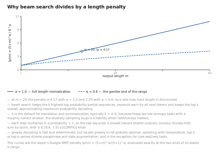
Figure 3. Why beam search divides by a length penalty.

4. Coverage: the repetition / dropping failure mode

Seq2seq generation has a characteristic failure the alignment view (Lesson 4) explains: because cross-attention is recomputed freely each step with no memory of what it already attended to, the decoder can attend to the same source span repeatedly (→ repetition, “the the the”) or never attend to some span (→ under-translation / dropped content). The classic fix is a coverage mechanism: maintain a running sum of attention given to each source position so far,

$$ \mathbf c^{t}=\sum_{t'=1}^{t-1}A_{t',:}\in\mathbb R^{n}\quad(\text{coverage vector}), $$

then either feed $\mathbf c^t$ into the attention computation so the model can see what it has covered, or add a coverage loss that penalizes attending to already-covered positions:

$$ \mathcal L_{\text{cov}}=\sum_{t}\sum_{j}\min\big(A_{tj},\,c^{t}_{j}\big). $$

Coverage was introduced for RNN attention (See et al.; Tu et al.) and the idea carries directly to transformer cross-attention. At transformer scale, large pretraining plus beam search with a repetition/length penalty often suffices, but coverage remains the principled account of why repetition and omission happen — uncontrolled re-attention to the source.

---

5. Copy mechanisms: when the output should reuse the input

Summarization and translation frequently need to reproduce exactly a token from the source — a name, a number, a rare or out-of-vocabulary word the decoder’s softmax would struggle to generate. The pointer-generator (See et al., 2017) addresses this by letting the model, at each step, either generate from the vocabulary or copy from the source by pointing at it through the cross-attention distribution. A learned soft gate $p_{\text{gen}}\in[0,1]$ mixes the two:

$$ P(w)=p_{\text{gen}}\,P_{\text{vocab}}(w)\;+\;(1-p_{\text{gen}})\!\!\sum_{j:\,x_j=w}\!\! A_{tj}, \qquad p_{\text{gen}}=\sigma(\mathbf w_h^\top\mathbf h_t+\mathbf w_c^\top\mathbf c_t+\mathbf w_q^\top\mathbf q_t+b). $$

The second term is literally the cross-attention weight on source positions whose token is $w$ — the alignment $A$ doubles as a copy distribution. This elegantly reuses the mechanism we already have: cross-attention both retrieves meaning (for generation) and points (for copying). Subword tokenization (BPE/SentencePiece) reduced the OOV pressure that originally motivated copying, so frontier models rely on it less, but it remains the clean answer to “the output must contain this exact source token.”

Learned / config / state

Quantity	Category
Frozen weights $\theta$, $p_{\text{gen}}$ gate (if trained)	[LEARNED], never change at inference
Strategy (greedy/beam/sampling), beam width $k$, length penalty $\alpha$, $T$/top-k/top-p, max length	[CONFIG]
$H_{\text{enc}}$, self-attn KV cache (grows), cross-attn KV cache (fixed), logits, coverage vector	[STATE]

---

Conclusion

Inference encodes once and decodes many: the bidirectional encoder produces $H_{\text{enc}}$ in a single pass, then the decoder generates autoregressively against it. The two-stack design yields two KV caches — a growing self-attention cache (output tokens) and a fixed cross-attention cache (computed once from $H_{\text{enc}}$ and never recomputed), making per-step conditioning on the input cheap. Beam search with length normalization is the seq2seq default because translation and summarization are low-entropy tasks with a roughly-correct answer. The alignment matrix $A$ from cross-attention explains and powers two seq2seq-specific tools: coverage (track cumulative attention to curb repetition and dropped content) and copy / pointer-generator mechanisms (point through $A$ to reproduce exact source tokens). Every knob is configuration; every buffer is transient state; $\theta$ is frozen — closing the train/infer loop opened in Lesson 8.

The mechanism is complete. Lesson 10 puts it to work: framing every task as text-to-text, fine-tuning for translation and summarization, measuring with BLEU and ROUGE, and shrinking the model by distillation into T5-small — and closes the course with the invariant that carried it.

---

← Lesson 8 — Training: Teacher Forcing · Course index · Next: Lesson 10 — Fine-Tuning & Distillation →

Appendices: A — Formulas · B — Architecture Comparison · C — Acronyms

---

The figures in this lesson follow the shared figure key , which explains what every shape, line style and colour means.