Lesson 10 — Fine-Tuning, Task Framing & Distillation
Technical course on encoder–decoder transformers — Lesson 10 of 10.
Recap of Lesson 9
Inference encodes once, decodes many: the encoder builds $H_{\text{enc}}$ in one pass; the decoder generates autoregressively with two KV caches — a growing self-attention cache and a fixed cross-attention cache. Beam search with length normalization is the seq2seq default; the alignment matrix $A$ powers coverage (anti-repetition) and copy/pointer-generator mechanisms. $\theta$ is frozen, every knob [CONFIG], every buffer [STATE]. We now take the pretrained model and make it useful: task framing, fine-tuning, evaluation, and compression.
1. Text-to-text: one interface for every task
T5’s organizing idea is that every NLP task can be cast as “text in → text out”, which is exactly the shape an encoder–decoder already has. Rather than attach task-specific heads (a classification head, a span head, a regression head — the encoder-only/BERT approach), T5 encodes the task itself into the input as a natural-language prefix, and reads the answer off the decoder as text:
$$ \begin{aligned} \texttt{"translate English to German: That is good."} &\;\to\; \texttt{"Das ist gut."}\\ \texttt{"summarize: \textless{}article…\textgreater{}"} &\;\to\; \texttt{"\textless{}summary…\textgreater{}"}\\ \texttt{"cola sentence: The course is jumps well."} &\;\to\; \texttt{"unacceptable"}\\ \texttt{"stsb sentence1: … sentence2: …"} &\;\to\; \texttt{"3.8"}\ (\text{a number, as text}). \end{aligned} $$The payoff is uniformity: the same model, same loss, same decoding handle translation, summarization, classification, and regression — only the data and the prefix change. Classification becomes “generate the class name”; regression becomes “generate the number as a string.” This is a [CONFIG]/data convention, not an architecture change — the cross-attention core of Lessons 4–5 is untouched. (BART, lacking this framing, is fine-tuned the more conventional way: feed source to the encoder, target to the decoder, with task-specific data.)
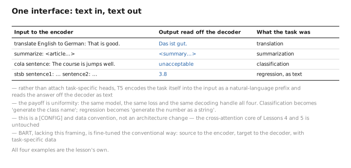
Figure 1. One interface: text in, text out.
2. Fine-tuning: same machinery, real pairs
Fine-tuning a pretrained encoder–decoder is mechanically identical to pretraining (Lessons 7–8) with two changes: the data is now labeled (input, output) pairs for the target task, and the corruption step is gone — the encoder reads the real source, the decoder is teacher-forced on the real target.
$$ \mathcal L_{\text{ft}}(\theta)=-\frac{1}{m}\sum_{t=1}^{m}\log P_\theta\big(y_t\mid y_{\lt t},\,x\big), $$with $(x,y)$ a translation pair (WMT), an (article, summary) pair (CNN/DailyMail, XSum), or a (task-prefixed input, answer) pair. All parameters are typically updated, though parameter-efficient methods (LoRA, adapters, prompt-tuning) apply unchanged — they are agnostic to whether the backbone is decoder-only or encoder–decoder. The learning rate is much smaller than pretraining, and far fewer steps are needed because the representations are already good; cross-attention now specializes from “reconstruct corrupted text” to “align source to target for this task.”
3. Measuring generation: BLEU and ROUGE
Cross-entropy/perplexity measure how well the model predicts the reference token-by-token, but seq2seq outputs are judged by whether the generated text matches a reference, allowing for many valid phrasings. Two n-gram overlap metrics dominate, and the choice tracks the task’s bias toward precision or recall.
BLEU (translation) is precision-oriented: of the n-grams the model produced, how many appear in the reference? It multiplies modified n-gram precisions (typically $n=1\dots4$) and applies a brevity penalty to stop the model gaming precision by emitting very short outputs:
$$ \text{BLEU}=\underbrace{\min\!\Big(1,\,e^{1-r/c}\Big)}_{\text{brevity penalty}}\cdot\exp\!\Big(\sum_{n=1}^{4} w_n\log p_n\Big), $$with $c$ the candidate length, $r$ the reference length, $p_n$ the modified n-gram precision. The brevity penalty is the metric-side analogue of the length normalization of Lesson 9 — both exist because probability-maximizing decoders are biased toward shortness.
ROUGE (summarization) is recall-oriented: of the reference’s n-grams (ROUGE-N) or its longest common subsequences (ROUGE-L), how many did the summary recover? Summarization cares that salient content is covered, so recall is the natural lens. Both metrics are crude (they reward surface overlap, not meaning) and are increasingly supplemented by learned metrics (BERTScore, COMET), but BLEU and ROUGE remain the reporting standard for translation and summarization respectively.
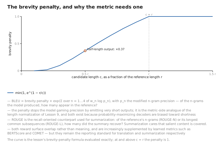
Figure 2. The brevity penalty, and why the metric needs one.
4. Distillation: shrinking the model
A pretrained encoder–decoder is large and its autoregressive decoder is the latency bottleneck at inference. Knowledge distillation trains a small student (e.g. T5-small, DistilBART) to imitate a large teacher, transferring capability into far fewer parameters. The student minimizes a blend of the true cross-entropy and a term matching the teacher’s softened distribution:
$$ \mathcal L_{\text{KD}}=(1-\lambda)\,\underbrace{\mathrm{CE}(y,\hat{\mathbf p}^{\,s})}_{\text{hard labels}} +\lambda\,T^2\,\underbrace{D_{\mathrm{KL}}\!\big(\hat{\mathbf p}^{\,t}_{T}\,\|\,\hat{\mathbf p}^{\,s}_{T}\big)}_{\text{soft teacher targets}}, $$where $\hat{\mathbf p}_T=\mathrm{softmax}(\mathbf z/T)$ are temperature-softened probabilities (the $T^2$ rescales the soft-target gradient to match the hard-label scale), and $\lambda$ is a [CONFIG] mixing weight. The teacher’s full distribution carries more information than the one-hot label — “the next token is Das with 0.7, Es with 0.2, …” tells the student about near-misses — so the student learns faster and better than from hard labels alone.
Two seq2seq-specific wrinkles. Sequence-level distillation (Kim & Rush, 2016) is the dominant practice: rather than match per-token distributions, run the teacher with beam search to produce high-quality target sequences, then train the student with ordinary teacher-forced CE on those teacher-generated targets — simpler and very effective for translation. And one can distill the stacks asymmetrically: DistilBART, for instance, keeps the full encoder but copies only a subset of decoder layers, because the autoregressive decoder dominates inference latency (it runs $m$ times; the encoder runs once, Lesson 9). The architecture’s compute asymmetry directly shapes how it is compressed.
Learned / config / state
| Quantity | Category |
|---|---|
| Fine-tuned/distilled student weights, $p_{\text{gen}}$ gate | [LEARNED] |
| Task prefixes, fine-tuning LR/steps, distillation $\lambda$ and $T$, beam width for seq-level KD | [CONFIG] |
| Teacher soft targets / generated sequences, logits, KV caches | [STATE] |
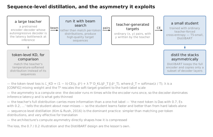
Figure 3. Sequence-level distillation, and the asymmetry it exploits.
Conclusion
A pretrained encoder–decoder becomes useful through text-to-text framing (T5): encode the task as an input prefix and read the answer as decoder text, so one model, loss, and decoder serve translation, summarization, classification, and regression alike. Fine-tuning is the training loop of Lesson 8 on real (input, output) pairs with no corruption; BLEU (precision, brevity-penalized) and ROUGE (recall, n-gram/LCS) score the generated text against references. Distillation — especially sequence-level KD, and asymmetric student designs that keep the encoder but thin the latency-dominant decoder — compresses the model into a T5-small or DistilBART. Throughout, the cross-attention core and the loss are untouched: only data, framing, and size change.
The whole course in one paragraph
A seq2seq task is the conditional map $P_\theta(y\mid x)=\prod_t P_\theta(y_t\mid y_{\lt t},x)$ (L1), met by two stacks: a bidirectional encoder that reads $x$ once into the memory $H_{\text{enc}}$ (L2) and a causal decoder that generates $y$ (L3) while reaching into that memory through cross-attention — queries from the decoder, keys/values from the encoder, a rectangular $m\times n$ alignment, the one new mechanism (L4). Assembled into three-sublayer decoder blocks (L5), the design is one point on a masking spectrum with the prefix-LM and decoder-only nearby (L6). It is pretrained by denoising — T5 span corruption, BART’s five noises (L7) — via teacher forcing, with the loss gradient routed through cross-attention to train both stacks jointly (L8); it is run by encoding once and decoding many against two KV caches, with beam search, coverage, and copy mechanisms (L9); and it is specialized and shrunk by fine-tuning and distillation (L10). One invariant carried all ten lessons: the encoder compresses context, the decoder generates conditioned on it, and cross-attention is the only new mechanism — plus the two inherited ones, training writes / inference reads and parameters learned, configuration chosen, state transient.
← Lesson 9 — Inference · Course index · Next: (none — final lesson)
Appendices: A — Formulas · B — Architecture Comparison · C — Acronyms
The figures in this lesson follow the shared figure key , which explains what every shape, line style and colour means.