Appendix A — A Field Guide to the Encoder Family
Technical course on encoder LLM mechanics — Appendix to Lessons 5 and 8.
Where this fits
This is a side-quest off Lessons 5 (the MLM objective) and 8 (pretraining dynamics). The names that get thrown around — RoBERTa, ALBERT, ELECTRA, DeBERTa, ModernBERT — are all answers to a limitation that a specific lesson identified. Rather than catalogue them flatly, this appendix organizes the family by what each model changed, along four axes that the lessons already gave us: the objective (Lesson 5), the masking/training (Lesson 8), the position scheme (Lesson 2), and the parameter budget (Lessons 2, 4). Read any row as “BERT, but with this fixed.”
A reading note on categories (Lesson 1’s framing): almost every choice below is [CONFIG] — architecture and training decided before the run. The weight matrices are [LEARNED]; the attention matrices and activations are [STATE]. When a model “is more efficient,” it is usually changing [CONFIG] (objective, masking, sharing) to extract more learning per FLOP, not inventing new kinds of numbers.
The baseline: BERT (2018)
Everything else is defined relative to this. Bidirectional Transformer encoder (Lessons 3–4), MLM + NSP objective (Lesson 5), WordPiece vocabulary of 30,522 (Lesson 2), learned-absolute positions capped at 512 (Lesson 2), post-LN blocks with GELU (Lesson 4). Two sizes: base ($N=12$, $d=768$, ~110M params) and large ($N=24$, $d=1024$, ~340M). Its weaknesses, in the order the later models attack them: under-trained, NSP is useless, only 15% of positions supervised, learned-absolute positions cap length, and embeddings eat a big share of parameters.
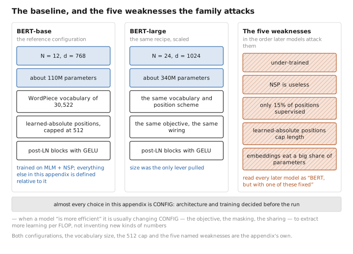
Figure 1. The baseline, and the five weaknesses the family attacks.
RoBERTa — “BERT was under-trained” (training fix, Lesson 8)
Same architecture, better recipe. RoBERTa changed only [CONFIG]: drop NSP entirely, use dynamic masking (fresh mask each epoch), train on ~10× more data (~160GB vs. ~16GB), much larger batches, longer schedules, and a byte-level BPE vocabulary. No architectural novelty — and it substantially beat BERT, proving the original was badly under-optimized. The lesson (8): for MLM’s low signal density, volume and training length are the cheapest large wins.
ALBERT — “shrink the parameters” (budget fix, Lessons 2, 4)
Two parameter-reduction tricks plus a better objective. Factorized embedding parameterization: instead of a $V\times d$ token embedding, use $V\times e$ then $e\times d$ with $e\ll d$, decoupling vocabulary size from hidden width (recall from Lesson 2 that embeddings are a large share of BERT-base). Cross-layer parameter sharing: reuse the same block weights across all $N$ layers, drastically cutting parameter count. And it replaces NSP with Sentence-Order Prediction (SOP) — distinguish correctly-ordered adjacent sentences from swapped ones, a genuinely harder coherence task than NSP (Lesson 5). Trades compute for memory: fewer parameters, but sharing can slow convergence.
DistilBERT — “make it deployable” (compression)
Knowledge distillation: train a small student (6 layers) to match a frozen BERT teacher’s output distribution (plus MLM and a cosine-embedding loss). Result: ~40% fewer parameters, ~60% faster inference, ~97% of BERT’s GLUE. Pure deployment play — same objective family, smaller body. The encoder analogue of distilling any large model.
ELECTRA — “supervise every position” (objective fix, Lessons 5, 8)
The most pointed attack on the 15% signal-density problem (Lesson 8). Instead of MLM, ELECTRA trains with replaced-token detection (RTD): a small generator replaces some tokens with plausible fakes, and the main encoder (the “discriminator”) classifies every token as original or replaced. Because the loss is defined at all positions, not just 15%, ELECTRA extracts far more signal per forward pass and reaches BERT-level quality with roughly a quarter of the compute. It is a GAN-flavored setup but trained with maximum likelihood, not adversarially.
$$ \mathcal L_{\text{RTD}}=-\sum_{i=1}^{n}\Big[\,\mathbb 1[\text{real}_i]\log D_i+\mathbb 1[\text{fake}_i]\log(1-D_i)\Big],\qquad D_i=\sigma(\mathbf w^\top H^{(N)}_{i,:}). $$The discriminator is what you keep and fine-tune; the generator is discarded.
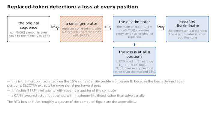
Figure 2. Replaced-token detection: a loss at every position.
DeBERTa — “better attention and positions” (mechanism fix, Lessons 2, 3)
Two ideas. Disentangled attention: represent each token by two vectors — content and relative position — and compute attention scores from content-to-content, content-to-position, and position-to-content terms separately, rather than baking position into one summed input vector (contrast Lesson 2’s additive scheme). Enhanced mask decoder: re-inject absolute position information near the output layer for the MLM head. DeBERTa (and DeBERTaV3, which swaps MLM for ELECTRA-style RTD) topped GLUE/SuperGLUE for a long stretch and is a common high-accuracy default.
ModernBERT (2024) — “a BERT with modern decoder engineering” (everything, all lessons)
The catch-up release. It imports the techniques the decoder world refined during the LLM boom: RoPE positions (Lesson 2) replacing learned-absolute, breaking the 512 ceiling to 8192 tokens; pre-LN blocks (Lesson 4) for stable training; GeGLU gated MLPs; FlashAttention and alternating local/global attention for speed; and training on far more data including code. The result is a drop-in encoder that is faster and far longer-context than BERT while retaining the bidirectional, MLM-trained, head-fine-tuned recipe of the whole course. It is the clearest evidence of the Lesson 10 point: most of these advances were decoder-pioneered and back-ported.
The family at a glance
| Model | Changed vs. BERT | Axis (lesson) | One-line payoff |
|---|---|---|---|
| BERT | — (baseline) | — | bidirectional MLM encoder |
| RoBERTa | drop NSP, dynamic mask, 10× data, big batches | training (8) | BERT was under-trained |
| ALBERT | factorized embeds, layer sharing, SOP | budget (2,4) | far fewer parameters |
| DistilBERT | distillation to 6 layers | compression | 60% faster, 97% quality |
| ELECTRA | replaced-token detection (all positions) | objective (5,8) | dense signal, ¼ compute |
| DeBERTa | disentangled attention, rel. positions | mechanism (2,3) | top GLUE accuracy |
| ModernBERT | RoPE→8192, pre-LN, GeGLU, FlashAttn, more+code data | all | modernized long-context encoder |
Takeaway. The encoder family is not a random zoo: each member fixes a named limitation from the lessons — under-training (RoBERTa), parameter bloat (ALBERT), inference cost (DistilBERT), signal density (ELECTRA), the additive-position bottleneck (DeBERTa), and the 512 ceiling plus dated engineering (ModernBERT). Hold the baseline in mind and every model reads as a one-line diff.
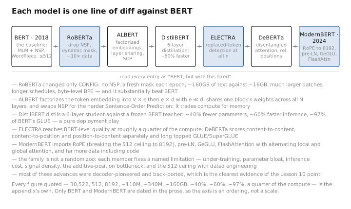
Figure 3. Each model is one line of diff against BERT.
← Course index · Extends Lesson 5 — Masked Language Modeling and Lesson 8 — Pretraining Dynamics
Appendices: A — Encoder Family · B — Encoder vs. Decoder Cheat Sheet · C — Acronyms
The figures in this lesson follow the shared figure key , which explains what every shape, line style and colour means.