Lesson 1 — The Big Picture: Encoder vs. Decoder

A 10-lesson technical course on the mechanics of encoder language models. Audience: comfortable with decoder-style LLMs at a high level; new to the specifics of encoders. Prerequisites: linear algebra (matrix products), multivariate calculus (gradients, the chain rule), and basic probability (distributions, expectation). We use standard notation throughout and define it as we go.

---

Course table of contents

#	Lesson	Core technical content
1	The Big Picture (this file)	The object $g(x;\theta):\mathcal V^{n}\to\mathbb R^{n\times d}$; bidirectional context; why there is no autoregressive factorization; the running decoder contrast
2	Tokenization & the Encoder Input	WordPiece; [CLS]/[SEP]/[MASK]; token + segment + position embeddings; learned-absolute positions
3	Bidirectional Self-Attention	$\mathrm{softmax}(QK^\top/\sqrt{d_k})V$ with no causal mask; the full $n\times n$ matrix; no KV cache; padding masks
4	The Encoder Block & Stack	Post-LN vs. pre-LN; the residual stream; contextual embeddings; how [CLS] summarizes a sequence
5	Masked Language Modeling	The MLM loss; 80/10/10 corruption; why bidirectionality demands denoising; NSP; masked cross-entropy
6	From Representations to Predictions	MLM head + weight tying; [CLS]/mean pooling; token- vs. sequence-level heads
7	Evaluating an Encoder	Masked cross-entropy; why perplexity fails; pseudo-perplexity; GLUE/SuperGLUE
8	Pretraining Dynamics	AdamW engine; the 15% signal-density problem; sequence packing; the RoBERTa recipe
9	Fine-Tuning Downstream	Classification, NER, span QA, sentence pairs; task heads; full FT vs. adapters
10	Practice & Landscape	Sentence-BERT; retrieval/RAG; RoBERTa/DeBERTa/ELECTRA/ModernBERT; encoder–decoder; which to choose
A	Appendix A — Encoder Family	BERT → ModernBERT, organized by what each model changed
B	Appendix B — Encoder vs. Decoder Cheat Sheet	Every contrast in the course, in one decision table
C	Appendix C — Acronyms	Every acronym and symbol, expanded in plain language

Two invariants run through every lesson and are worth stating before anything else:

• An encoder reads bidirectionally and emits representations, not a next-token distribution. Its output is a matrix $H\in\mathbb R^{n\times d}$ of context-aware vectors, one per input token, not a probability over the vocabulary.
• The pretraining objective must be a denoising task. Because every token can see every other, “predict the next token” is trivially solved by looking ahead. The model is instead trained to reconstruct corrupted input — this single fact reshapes the objective, the output head, the evaluation, and the fine-tuning story.

This course assumes you have met the decoder. If “autoregressive,” “KV cache,” or “cross-entropy next-token loss” are unfamiliar, read the companion decoder course first; here we treat the decoder as the known reference point and measure the encoder against it.

---

1. Two ways to be a language model

A decoder-only LLM is a function that reads the text so far and outputs a probability for every token in the vocabulary as the next token. Formally,

$$ f:\ \mathcal V^{\le n}\times\Theta\to\Delta^{V-1},\qquad \hat{\mathbf p}=f(x;\theta), $$

mapping a sequence to a point on the probability simplex $\Delta^{V-1}$ — a categorical distribution over the next token. Its defining property is the autoregressive factorization, the chain rule of probability:

$$ P_\theta(x_1,\dots,x_n)=\prod_{t=1}^{n}P_\theta(x_t\mid x_{\lt t}),\qquad x_{\lt t}:=(x_1,\dots,x_{t-1}). $$

Each factor conditions only on the past. That is not an aesthetic choice; it is what makes the factorization an exact identity, and it forces every token to be blind to its future.

An encoder drops that constraint entirely. Its job is not to predict what comes next but to represent what is here. It is a function

$$ \boxed{\ g:\ \mathcal V^{n}\times\Theta\to\mathbb R^{n\times d},\qquad H=g(x;\theta),\ } $$

mapping a length-$n$ token sequence to a length-$n$ sequence of $d$-dimensional vectors. Row $i$ of the output, $H_{i,:}\in\mathbb R^{d}$, is the contextual representation of token $i$: a vector that encodes what token $i$ means in this particular context, having looked at all the other tokens — both before and after it. The same word produces different output rows in different sentences (“bank” by a river vs. “bank” with money), which is the entire point.

Notice what is not in the output type. There is no $\Delta^{V-1}$, no distribution over the vocabulary, no “next token.” An encoder, on its own, predicts nothing. It produces a richer numerical description of the input that downstream heads (Lesson 6) then turn into predictions — a class label, a tag per token, an answer span, a similarity score. This is the sense in which decoders generate and encoders understand.

Invariant. A decoder’s native output is a distribution over the next token; an encoder’s native output is a matrix of contextual vectors. Everything else in this course follows from that difference.

Why “bidirectional” is the crux

The decoder’s causal constraint — position $t$ sees only $\le t$ — exists so that the training-time prediction at position $t$ cannot cheat by reading the answer ($x_t$ and beyond). An encoder has no such prediction to protect, so it lifts the constraint: position $i$ attends to all positions $1,\dots,n$. We will derive this precisely in Lesson 3, but the consequence is immediate and worth internalizing now: a representation that has seen the whole sentence is strictly more informative for understanding tasks than one that has seen only a prefix. The word “it” can be resolved by a noun that appears later; a sentiment can hinge on a final clause. Bidirectionality is what makes encoders the natural tool for classification, tagging, retrieval, and extraction.

---

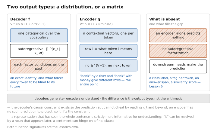
Figure 1. Two output types: a distribution, or a matrix.

2. The phases, and how they differ from the decoder’s

The decoder course’s central split — training writes $\theta$, inference reads $\theta$ — still holds. An encoder is trained by the same forward/backward/update loop, and at deployment its parameters are frozen. What changes is what each phase computes.

Training

Given a corpus $\mathcal D$, pretraining solves an empirical risk minimization

$$ \theta^\star=\arg\min_{\theta\in\mathbb R^{P}}\ \mathcal L(\theta), $$

but $\mathcal L$ is not the next-token loss. As §3 previews and Lesson 5 derives, it is a masked reconstruction loss: corrupt a fraction of the input, run the encoder, and score how well the model recovers the original tokens at the corrupted positions. The four-step loop (forward → backward → optimizer step → apply) is identical to the decoder’s; only the loss’s source differs.

Inference

Here the contrast is stark. A decoder at inference runs a loop: evaluate $f$ at the last position, sample a token, append it, evaluate again — $n$ forward passes to produce $n$ tokens, with a KV cache to avoid recomputation. An encoder at inference runs once: a single forward pass over the whole input produces all $n$ representations simultaneously. There is no token-by-token loop, no sampling, no KV cache, no temperature. You hand it a sequence; it hands you back a matrix.

Contrast with the decoder. Decoder inference is sequential and autoregressive ($O(n)$ forward passes, growing KV cache). Encoder inference is a single parallel pass ($1$ forward pass, no cache). This is why encoders are cheap to run as feature extractors and why they are useless as text generators.

---

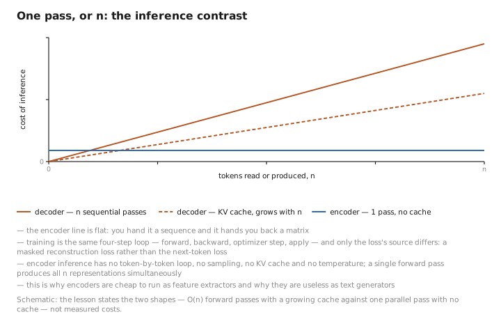
Figure 2. One pass, or n: the inference contrast.

3. The objective, previewed

The deepest difference is the training objective, so it is worth stating the logic now even though Lesson 5 does the math. A decoder is trained on next-token prediction precisely because it is causal: hiding the future is what makes the task non-trivial. Remove causality and that task collapses — if position $t$ can attend to $x_t$ itself, predicting $x_t$ is free. So a bidirectional model needs a different game.

The answer, introduced by BERT, is masked language modeling (MLM): replace a random ~15% of input tokens with a special [MASK] symbol (and some other corruptions, Lesson 5), run the full bidirectional encoder, and at each masked position predict the original token from its surrounding context. The loss is cross-entropy, but it is computed only at the masked positions:

$$ \mathcal L_{\text{MLM}}(\theta)=-\,\mathbb E_{x\sim\mathcal D}\ \sum_{i\in\mathcal M}\log P_\theta\!\big(x_i\mid x_{\setminus\mathcal M}\big), $$

where $\mathcal M$ is the set of masked positions and $x_{\setminus\mathcal M}$ is the sequence with those positions corrupted. Read it against the decoder’s loss: the decoder conditions on the past $x_{\lt t}$ and sums over all positions; the encoder conditions on the whole corrupted context and sums over only the masked positions. That contrast — what you condition on, and which positions contribute loss — is the spine of Lessons 5 through 7.

---

4. The three kinds of numbers (unchanged)

The number-categories from the decoder course carry over without modification, and we tag them identically throughout.

(a) Parameters $\theta$ — learned. Every weight matrix: the token embedding $E$, the new segment and position embeddings (Lesson 2), the attention projections $W_Q,W_K,W_V,W_O$, the MLP weights, the LayerNorm gains/shifts, and the MLM output projection. Initialized randomly, updated each step. Tagged [LEARNED].

(b) Configuration — chosen. Architectural: depth $N$, width $d$, heads $h$, MLP width $d_{ff}$, vocab $V$, max sequence length $n$. Process: learning rate, batch size, weight decay, and — uniquely for encoders — the masking rate (≈15%) and the masking recipe. Tagged [CONFIG].

(c) State — transient. Adam moments, cached activations, the attention matrices $A\in\mathbb R^{n\times n}$, and the logits at masked positions. Note what is absent relative to the decoder: there is no KV cache, because there is no autoregressive loop to cache for. Tagged [STATE].

Property	Parameters $\theta$	Configuration	State
Set by	gradient updates	humans / search	computed during a run
Encoder-specific members	segment embeddings, MLM head	masking rate, masking recipe	attention matrix $A$; no KV cache
Persists into deployed model?	yes	yes	no

---

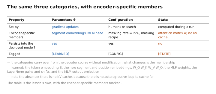
Figure 3. The same three categories, with encoder-specific members.

5. What an encoder is for

It helps to fix the use-cases now, because they motivate every design choice that follows. Decoders are deployed to produce text: chat, completion, code generation, agents. Encoders are deployed to score, classify, tag, and embed:

• Sequence classification — sentiment, spam, topic, intent (one label per input).
• Token classification — named-entity recognition, part-of-speech tagging (one label per token).
• Span extraction — extractive question answering (predict start/end positions in a passage).
• Sentence-pair tasks — entailment, paraphrase, semantic similarity.
• Embeddings & retrieval — turn a document or query into a single vector for search, clustering, or RAG.

Every one of these wants a rich, whole-context representation of given text, and none of them needs to generate new text. That is exactly the encoder’s contract.

---

Conclusion

An encoder language model is a function $g(x;\theta):\mathcal V^{n}\to\mathbb R^{n\times d}$ that maps a token sequence to a sequence of contextual representations, each informed by the entire input bidirectionally. It differs from a decoder at every level, and all the differences descend from one root: an encoder reads rather than writes. Because it is bidirectional it has no autoregressive factorization, so it cannot be trained on next-token prediction and is instead trained by masked reconstruction; because it emits representations rather than a next-token distribution it needs task heads to make predictions; because it makes no token-by-token loop it has no KV cache and runs in a single parallel forward pass; and because it does not generate, it is evaluated and fine-tuned differently. The same number-categories — [LEARNED], [CONFIG], [STATE] — and the same training engine apply throughout; what changes is the object, the objective, and the output.

The next lessons open the box from the bottom up, exactly as the decoder course did, but at each layer we will hold the decoder version up beside the encoder version. Lesson 2 starts at the boundary where text becomes numbers — and finds that an encoder’s input is built differently from a decoder’s from the very first token.

---

← Previous: (none — this is the first lesson) · Course index · Next: Lesson 2 — Tokenization & the Encoder Input →

Appendices: A — Encoder Family · B — Encoder vs. Decoder Cheat Sheet · C — Acronyms

---

The figures in this lesson follow the shared figure key , which explains what every shape, line style and colour means.